Aligning active Brownian particles — generic pairs API

Infer pairwise interaction forces in a system of aligning active Brownian particles (ABPs) using generic pair-interaction building blocks from SFI.bases.pairs.

First we simulate the ABP system using the pre-built ABP model, then save and reload the trajectory to demonstrate the I/O round-trip, and finally construct a generic pair-interaction basis for linear inference.

This example demonstrates:

1. Simulating a multi-particle ABP system with an example-local ABP helper (thin wrapper around SFI.bases.pairs).

2. Saving and loading trajectory data (CSV round-trip).

3. Constructing a generic Basis from heading_vector(), radial_pair_basis(), and angular_pair_basis().

4. Linear force inference using that basis.

5. Recovering the learned interaction kernels vs the true model.

Tags

synthetic · overdamped · multi-particle · linear · interactions

System: aligning active Brownian particles

Each particle has position \((x, y)\) and heading \(\theta\) — three degrees of freedom. The force includes:

• Self-propulsion: \(c_0\,\hat{e}_\theta\)

• Pairwise repulsion: short-range, radially repulsive: \(\varepsilon\, e^{-r/R_0}\,\hat{r}_{ij}\)

• Pairwise alignment: angular torque: \(A\,\sin(\Delta\theta)\,e^{-r/L_0}\)

Positions obey periodic boundary conditions.

N_particles = 60
Lx, Ly = 30.0, 30.0       # periodic box dimensions
Nsteps = 2000              # simulation length
dt_sim = 0.02              # integration time step
D_iso = 0.05               # isotropic diffusion coefficient
seed = 0
box = jnp.array([Lx, Ly])

# True model parameters
c0_true = 1.0       # self-propulsion speed
eps_true = 2.0       # repulsion strength
A_true = 0.5         # alignment strength
R0_true = 1.0        # repulsion length scale
L0_true = 2.0        # alignment length scale

theta_F_exact = dict(c0=c0_true, eps=eps_true, A=A_true,
                     R0=R0_true, L0=L0_true)

Simulating the true model

We build the ABP model from the helpers in _gallery_utils/abp.py (a thin composition of SFI.bases.pairs primitives). The result is a parametric state function (PSF) with named parameters c0, eps, A, R0, L0.

from _gallery_utils.abp import make_abp_align_psf
from SFI.langevin import OverdampedProcess

F_psf = make_abp_align_psf(dim=3)
proc = OverdampedProcess(F_psf, D=D_iso, extras_global={"box": box})
proc.set_params(theta_F=theta_F_exact)

# Random initial conditions: uniform in box, random headings
key = random.PRNGKey(seed)
key, kx, kth = random.split(key, 3)
X0_xy = random.uniform(kx, (N_particles, 2)) * jnp.array([Lx, Ly])
TH0 = random.uniform(kth, (N_particles,), minval=-jnp.pi, maxval=jnp.pi)
x0 = jnp.concatenate([X0_xy, TH0[:, None]], axis=1)

proc.initialize(x0)
key, sub = random.split(key)
coll = proc.simulate(dt=dt_sim, Nsteps=Nsteps, key=sub)

print(f"Trajectory: {coll.T} frames, "
      f"{coll.N} particles, dim={coll.d}")

Trajectory: 2000 frames, 60 particles, dim=3

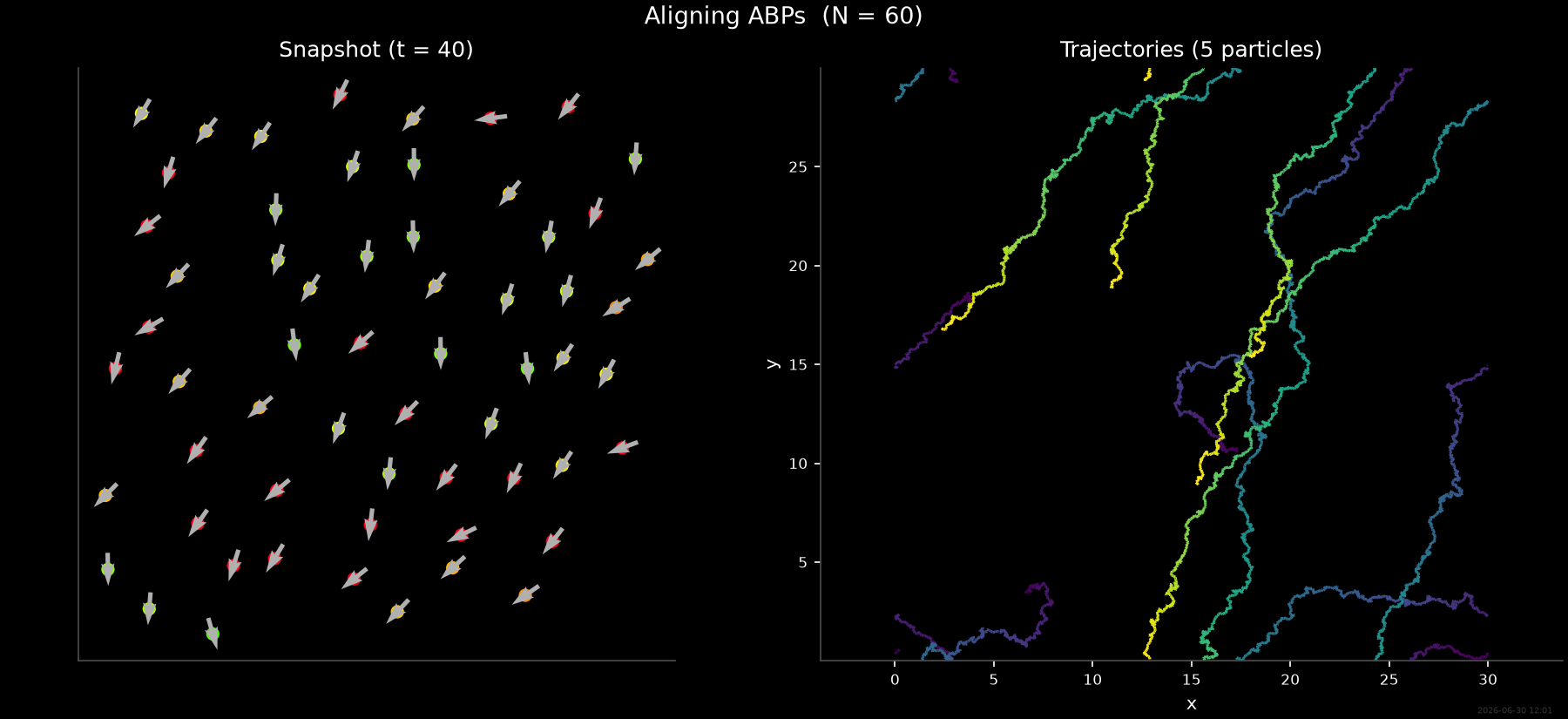
Simulation movie

Animation of the simulated ABP system. Particles are coloured by heading angle \(\theta\); white arrows show the propulsion direction.

Xfull = np.asarray(coll.X)  # full trajectory array (T × N × 3)

Saving and loading trajectory data

SFI trajectory collections can be serialised to CSV, Parquet, or HDF5 via save(). Global extras — here the periodic box — are embedded in a YAML header and survive the round-trip.

import os, tempfile
from SFI.trajectory import TrajectoryCollection

csv_path = os.path.join(tempfile.gettempdir(), "sfi_abp_demo.csv")
coll.save(csv_path, format="csv")

with open(csv_path) as f:
    for line in f.readlines()[:10]:
        print(line.rstrip())
print("  ...")

# Reload into a fresh collection and verify
coll_reloaded = TrajectoryCollection.load(csv_path)
print(f"\nOriginal:  T={coll.T}, N={coll.N}, d={coll.d}  →  Loaded: T={coll_reloaded.T}, N={coll_reloaded.N}, d={coll_reloaded.d}")
max_err = float(np.max(np.abs(coll_reloaded.X - coll.X)))
print(f"Max |ΔX| = {max_err:.1e}  (numerical round-trip error)")

# ---
# kind: overdamped
# dimension: 3
# pdepth: 1
# num_particles: 60
# x0:
# - - 0.21881461143493652
#   - 0.6267356872558594
#   - 2.5286648273468018
# - - 17.442794799804688
  ...

Original:  T=2000, N=60, d=3  →  Loaded: T=2000, N=60, d=3
Max |ΔX| = 7.5e-09  (numerical round-trip error)

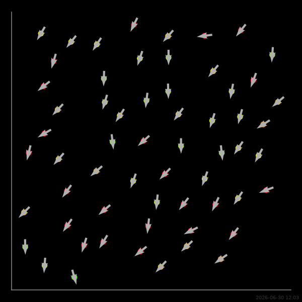
Particle snapshot

Final-frame snapshot with heading arrows (left) and individual particle trajectories (right). Positions are wrapped into the periodic box; particles are coloured by heading angle.

n_show = min(5, N_particles)  # trajectories to display

Building the pair-interaction basis

For inference, we construct a generic basis from building blocks in SFI.bases.pairs. The basis is deliberately over-complete — it contains many more radial kernels than the true model uses — so the linear solver must pick out the right combination.

1. Self-propulsion — heading_vector() gives the unit heading \((\cos\theta, \sin\theta, 0)\).

2. Radial repulsion — radial_pair_basis() with exponential- polynomial kernels.

3. Angular alignment — angular_pair_basis() with a \(\sin(\Delta\theta)\) coupling.

from SFI.bases.pairs import (
    angular_pair_basis,
    exp_poly_kernels,
    heading_vector,
    radial_pair_basis,
)
from SFI.statefunc import Basis

dim = 3  # (x, y, θ) per particle

# Radial kernels: r^n * exp(-r/L) for n ∈ {0,1}, L ∈ {0.5, 1, 2, 4}
repel_kernels = exp_poly_kernels(degrees=[0, 1], lengths=[0.5, 1.0, 2.0, 4.0])
align_kernels = exp_poly_kernels(degrees=[0, 1], lengths=[0.5, 1.0, 2.0, 4.0])

# Self-propulsion: (cos θ, sin θ, 0)
B_heading = heading_vector(dim=dim, angle_index=2)

# Radial pair repulsion → dispatched Basis (acts in xy-plane)
inter_repel = radial_pair_basis(
    repel_kernels, dim=dim,
    box="extras",
    spatial_dims=slice(0, 2),          # xy positions for distance
    embed_dim=dim, embed_axes=[0, 1],  # embed radial force into xy
)
B_repel = inter_repel.dispatch_pairs(
    symmetric=True, exclude_self=True,
    owners="focal", reducer="sum", return_as="basis",
)

# Angular alignment → dispatched Basis (acts on θ)
inter_align = angular_pair_basis(
    align_kernels, jnp.sin, dim=dim,
    angle_index=2, output_index=2,     # coupling: sin(Δθ) → force on θ
    box="extras",
    spatial_dims=slice(0, 2),
)
B_align = inter_align.dispatch_pairs(
    symmetric=True, exclude_self=True,
    owners="focal", reducer="sum", return_as="basis",
)

# Stack into one combined basis for inference
B_full = Basis.stack([B_heading, B_repel, B_align])

n_heading = B_heading.n_features
n_repel = B_repel.n_features
n_align = B_align.n_features

Linear force inference

Standard infer_force_linear() recovers the interaction coefficients in a single linear solve — no gradient-based optimisation needed.

from SFI import OverdampedLangevinInference
from SFI.utils import plotting

# Create inference object from the trajectory collection
inf = OverdampedLangevinInference(coll)

# Estimate diffusion coefficient
inf.compute_diffusion_constant(method="WeakNoise")

# Solve for force coefficients (one-shot linear solve)
inf.infer_force_linear(B_full, M_mode="Ito", G_mode="rectangle")

# Estimate coefficient uncertainty (populates force_coefficients_covariance)
inf.compute_force_error()

# Compare to exact model for quantitative error metrics
inf.compare_to_exact(model_exact=proc, maxpoints=2000)
inf.print_report()

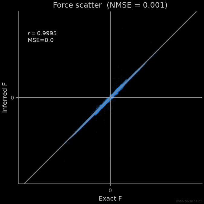
nmse_abp = float(inf.NMSE_force)  # reused in the force-scatter title

  --- StochasticForceInference Report ---
Average diffusion tensor:
 [[ 4.9648169e-02 -1.6120239e-05 -1.0172471e-04]
 [-1.6120215e-05  4.9877696e-02 -1.6907154e-04]
 [-1.0172469e-04 -1.6907144e-04  4.9801379e-02]]
Measurement noise tensor:
 [[-1.5219006e-04 -8.3711362e-05  5.3390534e-07]
 [-8.3711362e-05 -2.2979152e-04 -3.4853206e-06]
 [ 5.3390534e-07 -3.4853210e-06 -8.2759789e-06]]
Force estimated information: 12177.7060546875
Force: estimated normalized mean squared error (sampling only): 0.0005337358762452214
Normalized MSE (force):     0.0007
Normalized MSE (diffusion): 0.0000

  Force Coefficient Table
  ──────────────────────────────────────────────────────────────────────────
  #    Label               Coefficient       Std.Err     SNR  Sig
  ──────────────────────────────────────────────────────────────────────────
  0    e_heading           9.95722e-01   6.56048e-03   151.8  ***
  1    r^0·exp(-r/0.5)     3.34897e+00   1.93552e+00     1.7  ·
  2    r^0·exp(-r/1)      -4.99166e+00   2.76279e+00     1.8  ·
  3    r^0·exp(-r/2)      -1.84840e+00   5.16968e-01     3.6  *
  4    r^0·exp(-r/4)       3.16612e-02   1.45463e-01     0.2  ·
  5    r^1·exp(-r/0.5)     4.37969e+00   3.73906e+00     1.2  ·
  6    r^1·exp(-r/1)       2.38924e+00   4.90655e-01     4.9  *
  7    r^1·exp(-r/2)       1.11856e-01   4.70822e-02     2.4  *
  8    r^1·exp(-r/4)      -2.23570e-02   1.33291e-02     1.7  ·
  9    g·r^0·exp(-r/0.5)  -4.35410e+01   3.46116e+00    12.6  **
  10   g·r^0·exp(-r/1)     2.50350e+01   4.92693e+00     5.1  *
  11   g·r^0·exp(-r/2)     2.55251e+01   4.97670e-01    51.3  **
  12   g·r^0·exp(-r/4)     3.83326e+00   8.76765e-02    43.7  **
  13   g·r^1·exp(-r/0.5)  -5.32409e+01   7.19212e+00     7.4  *
  14   g·r^1·exp(-r/1)    -3.07139e+01   1.00916e+00    30.4  **
  15   g·r^1·exp(-r/2)    -4.90880e+00   6.85575e-02    71.6  **
  16   g·r^1·exp(-r/4)    -1.75143e-01   8.78098e-03    19.9  **
  ──────────────────────────────────────────────────────────────────────────
  17/17 basis functions in support, sig: 12* / 7** / 1*** (|SNR| ≥ 2 / 10 / 100)
  (Std.err. reflects sampling error only; discretization bias is not included.)

Force scatter: exact vs inferred

All force components (translational and angular) along the trajectory, plotted as a scatter. Points near the diagonal indicate good inference.

# The force is a multi-particle interacting field (per-frame neighbour
# structure + the ``box`` extra), so evaluate it per frame on ``coll.X``
# rather than via force_comparison_arrays (which flattens to single points).
Xe = proc.force_sf(coll.X, extras={"box": box})
Xi = inf.force_inferred(coll.X, extras={"box": box})

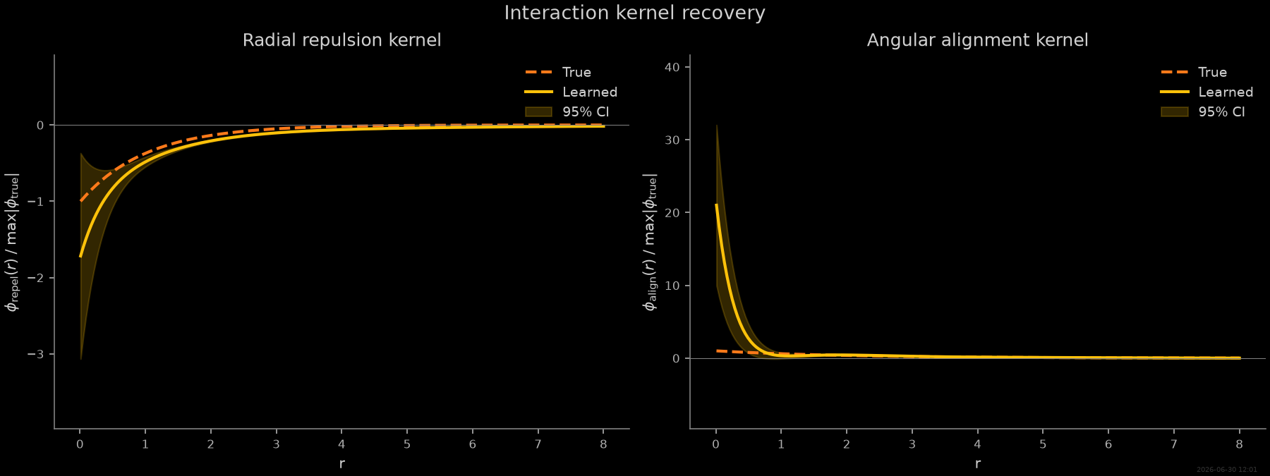
Recovered interaction kernels

The inferred coefficients weight the radial kernels. Summing \(\sum_k c_k \phi_k(r)\) reconstructs the effective radial interaction shape. Shaded bands show 95 % confidence intervals derived from the coefficient covariance (see kernel_predict_ci()).

from SFI.inference import kernel_predict_ci

# Extract inferred coefficients and covariance sub-blocks for each basis block
c_heading, _ = inf.coeff_block(B_heading, field='force')
c_repel, cov_repel = inf.coeff_block(B_repel, field='force')
c_align, cov_align = inf.coeff_block(B_align, field='force')

# True coefficient vectors in the generic-basis coordinate system
# Kernel ordering from exp_poly_kernels(degrees=[0,1], lengths=[0.5,1,2,4]):
#   k=0: r⁰·e⁻ʳ/0.5   k=1: r⁰·e⁻ʳ/1   k=2: r⁰·e⁻ʳ/2   k=3: r⁰·e⁻ʳ/4
#   k=4: r¹·e⁻ʳ/0.5   k=5: r¹·e⁻ʳ/1   k=6: r¹·e⁻ʳ/2   k=7: r¹·e⁻ʳ/4
idx_repel = 1  # r⁰·e⁻ʳ/R₀ with R₀=1.0
idx_align = 2  # sin(Δθ)·r⁰·e⁻ʳ/L₀ with L₀=2.0

true_c_repel = np.zeros(n_repel)
true_c_repel[idx_repel] = -eps_true
true_c_align = np.zeros(n_align)
true_c_align[idx_align] = A_true

# Compute kernel profiles with confidence intervals
r_eval = np.linspace(0.01, 8.0, 200)
ci_repel = kernel_predict_ci(r_eval, repel_kernels, c_repel, cov_repel)
ci_align = kernel_predict_ci(r_eval, align_kernels, c_align, cov_align)

# True kernel profiles (for comparison)
true_repel = true_c_repel @ ci_repel["phi"]
true_align = true_c_align @ ci_align["phi"]

Inferred self-propulsion

The heading coefficient recovers the active thrust magnitude \(c_0\):

Bootstrapped trajectory

Simulating from the inferred model and comparing emergent collective behaviour is a powerful qualitative validation for multi-particle systems.

# Run a bootstrap simulation from the inferred coefficients
key_boot = random.PRNGKey(seed + 77)
proc_boot = inf.simulate_bootstrapped_trajectory(key_boot, simulate=False)
proc_boot.set_extras(extras_global={"box": box})
proc_boot.initialize(x0)                    # same initial conditions
key_boot, sub_boot = random.split(key_boot)
coll_boot = proc_boot.simulate(dt=dt_sim, Nsteps=Nsteps, key=sub_boot)

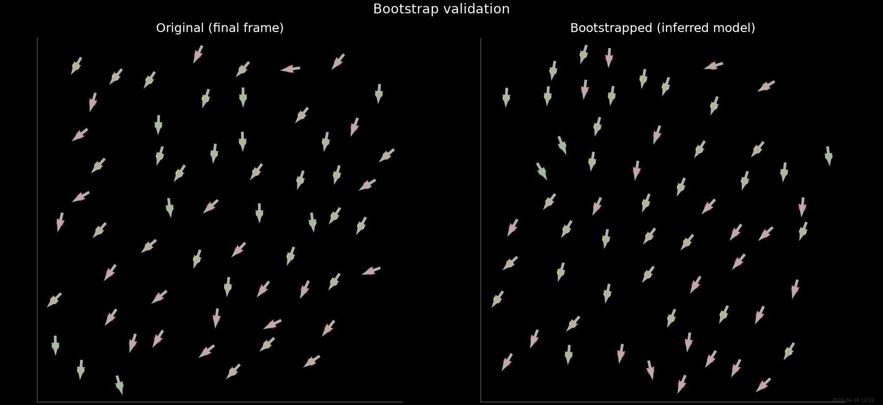
Bootstrap comparison movie

Side-by-side animation of the original trajectory (left) and a trajectory simulated from the inferred model (right). Both start from the same initial conditions.

Xboot_full = np.asarray(coll_boot.X)

Both simulations start from the same initial conditions. Visual similarity confirms the inferred model captures the collective dynamics.

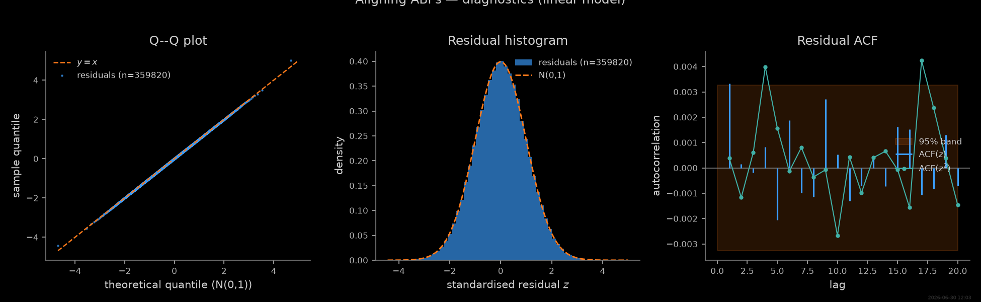
Diagnostics

assess() computes standardised Euler residuals pooled across all particles and spatial components (\(N_\mathrm{obs} \approx N_\mathrm{particles} \times T \times d\)), giving high statistical power even from a short trajectory. All three force channels — translational \((x,y)\) and angular \((\theta)\) — are pooled into a single residual vector.

The linear basis is over-complete by design, so the NMSE should be small but the coefficient z-scores for unused kernels will be near zero.

from SFI.diagnostics import assess, plot_summary

report = assess(inf, level="standard")
report.print_summary()

=== SFI diagnostics report ===
backend  : linear
regime   : OD
n_obs    : 119940  n_particles: 60  d: 3
level    : standard

-- Residuals --
  mean = +0.0003  std = 0.9988  skew = -0.005  kurt-3 = -0.000  (n=359820)
  ✓ normality ks                 stat=0.00143   p=0.454
  ✓ autocorr  ljung_box          stat=14.9      p=0.783
  ✓ autocorr  ljung_box_squared  stat=21        p=0.4
  predicted NMSE = 0.000534  realised NMSE = 0  χ² z = -1.00 (|z|>5 ⇒ bias)

-- Flags --
  (no issues at α = 0.01)

Thumbnail

Dedicated single-panel figure for the gallery thumbnail.

stamp_output()

examples/gallery/abp_align_demo.py:570: UserWarning: The figure layout has changed to tight
  plt.tight_layout()
[Generated: 2026-06-30 12:03]

🏷 Tags: synthetic, overdamped, multi-particle, linear, interactions