Overdamped or underdamped? Classifying dynamics from data

Before fitting a force, you must choose an engine: OverdampedLangevinInference assumes first-order (overdamped) dynamics, UnderdampedLangevinInference assumes second-order (inertial) dynamics. SFI.classify_dynamics() reads the data and decides which regime you are in — directly from positions, with no velocities required.

The discriminator is the lag-resolved displacement covariance \(C_k = \langle \Delta x_t \cdot \Delta x_{t+k}\rangle\). Two facts make it robust:

1. White localization noise touches only \(C_0\) and \(C_1\) (it adds \(+2\sigma^2\), \(-\sigma^2\), and exactly 0 at lag \(\ge 2\)), so lag-2 statistics are measurement-noise-immune.

2. A force field cannot fake inertia: scanning \(\Delta t\) separates the overdamped force confound (which vanishes as \(\Delta t\to0\)) from genuine momentum persistence (which saturates).

This demo classifies an overdamped double-well and an underdamped damped oscillator under the same heavy localization noise, then turns to the two cases the method must handle honestly: a coarsely-sampled inertial particle whose momentum is only half-resolved (verdict: inconclusive), and a driven, non-equilibrium 2D system it must still call overdamped.

Tags

diagnostics · overdamped · underdamped · 1D · 2D · non-equilibrium · synthetic

Simulate an overdamped and an underdamped trajectory

The overdamped process is a double well \(F(x) = x - x^3\); the underdamped one is a damped harmonic oscillator \(\dot v = -k x - \gamma v + \sqrt{2D}\,\xi\) with momentum relaxation time \(\tau_v = 1/\gamma = 1\). Both are sampled finely enough to resolve the (in)existence of momentum.

from SFI import classify_dynamics
from SFI.bases.constants import identity_matrix_basis
from SFI.bases import unit_axes, x_components
from SFI.diagnostics import plot_dynamics_order
from SFI.langevin import OverdampedProcess, UnderdampedProcess
from SFI.statefunc.factory import make_basis

# Overdamped double well, F(x) = x - x^3 (compositional).
(_x,) = x_components(1)
(_ex,) = unit_axes(1)
proc_od = OverdampedProcess((_x - _x * _x * _x) * _ex, D=0.15)
proc_od.initialize(jnp.array([0.5], dtype=jnp.float32))
coll_od = proc_od.simulate(
    dt=0.02, Nsteps=12000, key=random.PRNGKey(0), prerun=200, oversampling=10
)

# Underdamped damped harmonic oscillator, F(x, v) = -k x - gamma v.
k, gamma = 1.0, 1.0


def damped_oscillator(x, *, v, mask=None):
    return jnp.array([-k * x[0] - gamma * v[0]])


F_ud = make_basis(damped_oscillator, dim=1, rank=1, n_features=1, needs_v=True)
proc_ud = UnderdampedProcess(F_ud.to_psf(), D=identity_matrix_basis(1).to_psf())
proc_ud.set_params(theta_F={"coeff": jnp.array([1.0])}, theta_D={"coeff": jnp.array([1.0])})
proc_ud.initialize(jnp.array([1.0], dtype=jnp.float32), v0=jnp.array([0.0], dtype=jnp.float32))
coll_ud = proc_ud.simulate(
    dt=0.02, Nsteps=12000, key=random.PRNGKey(1), prerun=200, oversampling=10
)

Degrade both with the same heavy localization noise

Localization noise is the classic confound: it adds a strong negative one-step correlation that can masquerade as (or mask) the dynamics. Here \(\sigma = 0.06\) is comparable to a single step.

sigma = 0.06
coll_od_noisy = coll_od.degrade(noise=sigma, seed=10)
coll_ud_noisy = coll_ud.degrade(noise=sigma, seed=11)

Classify

classify_dynamics() runs the noise-immune scaling test, the parametric covariance fit (recovering \(\tau_v\), \(\sigma\), \(D\)), and an overdamped-fit residual-autocorrelation cross-check.

report_od = classify_dynamics(coll_od_noisy)
report_ud = classify_dynamics(coll_ud_noisy)

print("\n### Overdamped double well (with localization noise) ###")
report_od.print_summary()

print("\n### Underdamped damped oscillator (with localization noise) ###")
report_ud.print_summary()

### Overdamped double well (with localization noise) ###

=== SFI dynamics-order classification ===
verdict : OD
sampling: d=1, dt in [0.02, 0.64] over 6 strides

-- parametric fit (diffusion + inertia + localization) --
  tau_v = 1/gamma = 0.002306   (momentum relaxation time)
  <v^2> = 0.00938   D = 0.1113   sigma_loc = 0.06971
  AICc(OD) - AICc(UD) = -6.28   (>0 favours inertia)   V/stderr = 0.00

-- model-free scaling (noise-immune at lag>=2) --
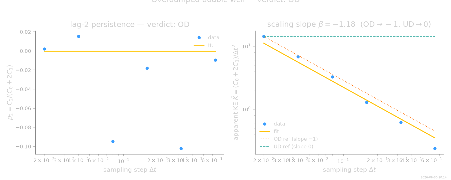
  rho2(finest dt) = 0.002   (OD -> 0, UD -> positive)
  apparent-KE log-log slope = -1.18   (OD -> -1, UD -> 0)

-- cross-check (OD-fit residual autocorrelation) --
  Ljung-Box p = 5.40e-02   (small => overdamped model leaves structure)


### Underdamped damped oscillator (with localization noise) ###

=== SFI dynamics-order classification ===
verdict : UD
sampling: d=1, dt in [0.02, 0.64] over 6 strides

-- parametric fit (diffusion + inertia + localization) --
  tau_v = 1/gamma = 0.4703   (momentum relaxation time)
  <v^2> = 0.9914   D = 2.371e-17   sigma_loc = 0.0576
  AICc(OD) - AICc(UD) = +51.53   (>0 favours inertia)   V/stderr = 7.05

-- model-free scaling (noise-immune at lag>=2) --
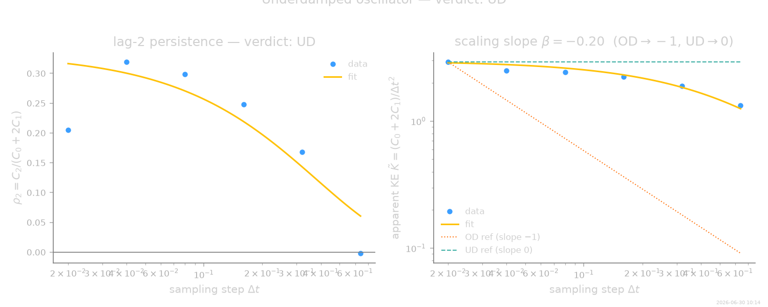
  rho2(finest dt) = 0.205   (OD -> 0, UD -> positive)
  apparent-KE log-log slope = -0.20   (OD -> -1, UD -> 0)

-- cross-check (OD-fit residual autocorrelation) --
  Ljung-Box p = 0.00e+00   (small => overdamped model leaves structure)

Visualise the overdamped verdict

Left: the noise-immune lag-2 correlation \(\rho_2\) stays near zero. Right: the apparent kinetic energy grows as \(1/\Delta t\) (slope \(-1\)) — the signature of a rough, non-differentiable (overdamped) path.

fig_od = plot_dynamics_order(report_od)
fig_od.suptitle(f"Overdamped double well — verdict: {report_od.verdict}", y=1.02)

Text(0.5, 1.02, 'Overdamped double well — verdict: OD')

Visualise the underdamped verdict

Now \(\rho_2\) rises toward a positive plateau as \(\Delta t\) shrinks (momentum persistence), and the apparent kinetic energy flattens (slope \(\to 0\)) — a smooth, differentiable (underdamped) path. The localization noise, confined to lags 0 and 1, never enters this verdict.

fig_ud = plot_dynamics_order(report_ud)
fig_ud.suptitle(f"Underdamped oscillator — verdict: {report_ud.verdict}", y=1.02)

Text(0.5, 1.02, 'Underdamped oscillator — verdict: UD')

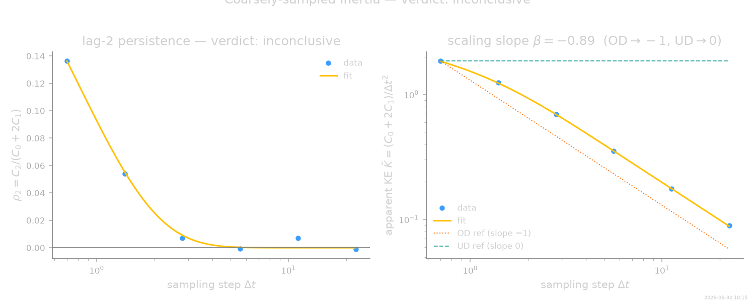
Coarse sampling: an honest inconclusive

The underdamped verdict above is only possible because momentum was resolved — sampled finely compared with \(\tau_v\). What if it is not? Here is a freely diffusing inertial particle (velocity relaxes at rate \(\gamma = 1\), no confining force, so it matches the classifier’s covariance model exactly) sampled coarsely at \(\Delta t = 0.7\), so \(\gamma\,\Delta t \approx 0.7\) and momentum is barely half-resolved.

Note the large sample size: at coarse sampling the velocity signal is weak, so many samples are needed before the fit can detect inertia at all — a practical cost of operating near the resolution boundary.

def free_inertial(x, *, v, mask=None):
    return jnp.array([-1.0 * v[0]])  # F = -gamma v, gamma = 1; no confining force


F_free = make_basis(free_inertial, dim=1, rank=1, n_features=1, needs_v=True)
proc_free = UnderdampedProcess(F_free.to_psf(), D=identity_matrix_basis(1).to_psf())
proc_free.set_params(theta_F={"coeff": jnp.array([1.0])}, theta_D={"coeff": jnp.array([1.0])})
proc_free.initialize(jnp.zeros(1, dtype=jnp.float32), v0=jnp.zeros(1, dtype=jnp.float32))
coll_coarse = proc_free.simulate(
    dt=0.7, Nsteps=500_000, key=random.PRNGKey(1), prerun=500, oversampling=10
)

# cross_check refits a full overdamped model; skip it on this large dataset.
# The verdict rests on the noise-immune scaling test and the parametric fit.
report_inc = classify_dynamics(coll_coarse, cross_check=False)

print("\n### Freely diffusing inertial particle, coarsely sampled ###")
report_inc.print_summary()

### Freely diffusing inertial particle, coarsely sampled ###

=== SFI dynamics-order classification ===
verdict : inconclusive
sampling: d=1, dt in [0.7, 22.4] over 6 strides

-- parametric fit (diffusion + inertia + localization) --
  tau_v = 1/gamma = 0.9819   (momentum relaxation time)
  <v^2> = 0.9984   D = 0.006267   sigma_loc = 1.73e-07
  AICc(OD) - AICc(UD) = +99.99   (>0 favours inertia)   V/stderr = 4.86

-- model-free scaling (noise-immune at lag>=2) --
  rho2(finest dt) = 0.136   (OD -> 0, UD -> positive)
  apparent-KE log-log slope = -0.89   (OD -> -1, UD -> 0)

  Note: momentum only marginally resolved (gamma*dt_min ~ 0.71); sample finer than tau_v to decide.

The classifier abstains rather than guess. The parametric fit still detects inertia (a large AICc gain), but the noise-immune lag-2 persistence at the finest step has decayed into the gray zone between the overdamped and underdamped thresholds. The summary reports \(\gamma\,\Delta t\) and tells you to sample finer than \(\tau_v\) to decide.

fig_inc = plot_dynamics_order(report_inc)
fig_inc.suptitle(f"Coarsely-sampled inertia — verdict: {report_inc.verdict}", y=1.02)

Text(0.5, 1.02, 'Coarsely-sampled inertia — verdict: inconclusive')

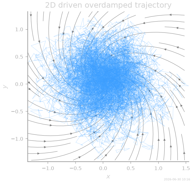
Beyond 1D: a driven, non-equilibrium 2D system

The test pools spatial components isotropically, so it works in any dimension. Here is a 2D overdamped particle in a harmonic trap with a non-conservative rotational force, \(\mathbf{F}(\mathbf{x}) = -k\,\mathbf{x} + \omega\,(\hat z \times \mathbf{x})\) — a detailed-balance-breaking curl that drives a steady probability current, the kind of active/driven system SFI targets. Being driven out of equilibrium is not the same as being inertial: a first-order force cannot manufacture momentum, so the verdict should stay OD.

x0, x1 = x_components(2)
e0, e1 = unit_axes(2)
k2, omega = 1.0, 1.0
F_rot = (-k2 * x0 - omega * x1) * e0 + (-k2 * x1 + omega * x0) * e1
proc_2d = OverdampedProcess(F_rot, D=0.15)
proc_2d.initialize(jnp.array([0.5, 0.0], dtype=jnp.float32))
coll_2d = proc_2d.simulate(
    dt=0.02, Nsteps=12000, key=random.PRNGKey(0), prerun=200, oversampling=10
)
coll_2d_noisy = coll_2d.degrade(noise=sigma, seed=12)

report_2d = classify_dynamics(coll_2d_noisy)

print("\n### 2D overdamped with a rotational (curl) force ###")
report_2d.print_summary()

### 2D overdamped with a rotational (curl) force ###

=== SFI dynamics-order classification ===
verdict : OD
sampling: d=2, dt in [0.02, 0.64] over 6 strides

-- parametric fit (diffusion + inertia + localization) --
  tau_v = 1/gamma = 0.0018   (momentum relaxation time)
  <v^2> = 0.5659   D = 0.1348   sigma_loc = 0.06497
  AICc(OD) - AICc(UD) = -6.28   (>0 favours inertia)   V/stderr = 0.00

-- model-free scaling (noise-immune at lag>=2) --
  rho2(finest dt) = 0.020   (OD -> 0, UD -> positive)
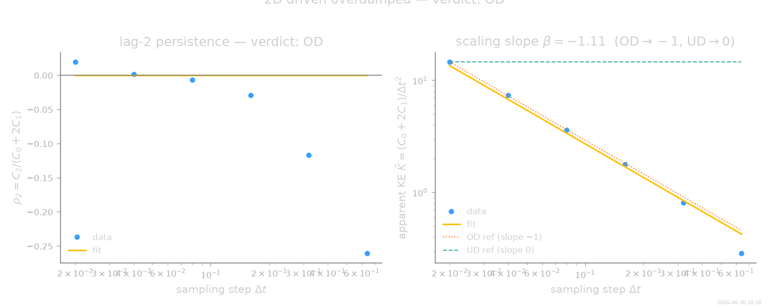
  apparent-KE log-log slope = -1.11   (OD -> -1, UD -> 0)

-- cross-check (OD-fit residual autocorrelation) --
  Ljung-Box p = 3.59e-01   (small => overdamped model leaves structure)

The force field is a rotational current (grey streamlines) that breaks detailed balance; the noisy overdamped path (blue) fills the trap around it. The circulation is real — yet every increment is still non-differentiable, which is what the verdict keys on.

fig_traj, ax_traj = plt.subplots(figsize=(4.2, 4.0))
# Deterministic force field F = -k x + omega (z x x), drawn for context.
stream_field(
    coll_2d_noisy, proc_2d.force_sf, N=25,
    color="#808080", linewidth=0.5, density=0.8, arrowsize=0.7, ax=ax_traj,
)
phase2d(
    coll_2d_noisy, dims=(0, 1), color=SFI_COLORS["data"],
    linewidth=0.3, alpha=0.5, ax=ax_traj,
)
ax_traj.set_xlabel("$x$")
ax_traj.set_ylabel("$y$")
ax_traj.set_title("2D driven overdamped trajectory")

Text(0.5, 1.0, '2D driven overdamped trajectory')

And the verdict: still OD. The rotational drive leaves the lag-2 persistence at zero — driving is not inertia.

fig_2d = plot_dynamics_order(report_2d)
fig_2d.suptitle(f"2D driven overdamped — verdict: {report_2d.verdict}", y=1.02)

plt.show()

Takeaways

• The verdict is built from lag-2 statistics, which white localization noise cannot reach — so heavy noise that dominates \(C_0\) does not flip the classification.

• The \(\Delta t\)-scan is what defeats the force confound: an overdamped force only adds an \(\mathcal{O}(\Delta t^2)\) correction to a variance that grows like \(\Delta t\), so it vanishes under refinement, whereas inertia saturates.

• When momentum is only marginally resolved (\(\gamma\,\Delta t \sim 1\), the coarse-sampled case above) the classifier honestly returns "inconclusive" rather than guessing — and detecting even that marginal inertia takes a large sample.

• It pools spatial components isotropically, so it works in any dimension; and because it keys on trajectory smoothness, a driven non-equilibrium force (the 2D rotational case) is correctly read as overdamped — driving is not inertia.

stamp_output()

[Generated: 2026-06-30 10:16]

🏷 Tags: diagnostics, overdamped, underdamped, 1D, 2D, non-equilibrium, synthetic