Discovering Toner–Tu hydrodynamics from agent-based flocking

Note

Uses the experimental SPDE toolbox — see SPDE (spatial fields) — experimental.

A polar active-matter “round trip”: simulate 10 000 self-propelled particles with Vicsek-like alignment, coarse-grain their positions and orientations into continuum fields (ρ, m_x, m_y), and let SFI + PASTIS discover the governing SPDE — without ever telling it which terms to expect.

Pipeline:

1. Microscopic ABPs (SFI.langevin.OverdampedProcess + chunked neighbor-list rebuilds): self-propulsion + soft repulsion + short-range polar alignment, tuned to the banded flocking regime.

2. Coarse-graining (Gaussian-smoothed bilinear deposition, examples._gallery_utils.coarse_grain.coarse_grain_polar()): particles → density ρ and polar momentum m = ρ⟨\hat e_θ⟩ on a periodic 64×64 grid.

3. Overcomplete SPDE basis (GridLayout with one ScalarSector for ρ and one spatial VectorSector for m): ~30 candidate terms covering continuity, polar Landau ordering, Frank elasticity, advection, and pressure-like density gradients.

4. Linear inference + PASTIS sparsification recovers the dominant Toner–Tu terms.

5. Bootstrap the inferred SPDE from random initial conditions and compare its bands to the agent-based ones.

Tags

synthetic · overdamped · multi-particle · linear · spde · pastis · interactions

Microscopic flocking model

Each agent carries position \((x_i, y_i)\) and heading \(\theta_i\). The force on the 3-vector state \((x, y, \theta)\) is

\[\mathbf F_i = \underbrace{c_0\, \hat e_{\theta_i}}_{\text{propulsion}} \;+\; \underbrace{\sum_j (-\varepsilon)\,e^{-r_{ij}/R_0}\, \hat r_{ij}}_{\text{soft repulsion}} \;+\; \underbrace{\hat z\sum_j A\,e^{-r_{ij}/L_a}\, \sin(\theta_j - \theta_i)}_{\text{Vicsek alignment}}\]

acting on \((x, y, \theta)\) respectively, plus rotational noise. We work in the banded flocking regime: high alignment, low rotational noise — propagating density bands aligned along the mean heading direction emerge spontaneously.

from SFI.bases.pairs import (
    angle_coupling,
    heading_vector,
    pair_direction,
    parametric_radial_kernel,
)
from SFI.langevin import OverdampedProcess
from SFI.langevin.chunked import simulate_chunked
from SFI.statefunc import Basis
from SFI.utils.neighbors import make_neighbor_extras

# ── physical parameters ──
N_particles = 10_000
Lx = Ly     = 64.0
Nsteps      = 1500
dt_sim      = 0.05
seed        = 7

# Particle force parameters (tuned for banded regime)
c0_true   = 0.50    # self-propulsion speed
eps_true  = 2.00    # repulsion strength
R0_true   = 0.50    # repulsion length
A_true    = 1.20    # alignment torque amplitude
La_true   = 1.50    # alignment kernel length

# Anisotropic noise: low translational, moderate rotational
D_xy      = 0.005
D_theta   = 0.10
D_matrix  = jnp.diag(jnp.array([D_xy, D_xy, D_theta]))

# Neighbor-list parameters
# cutoff = 3.0 captures repulsion (R0=0.5, exp(-6) ~ 2e-3) and alignment
# (La=1.5, exp(-2) ~ 0.13) tails to good accuracy.
cutoff = 3.0
skin   = 1.5
rebuild_every = 5

box    = jnp.array([Lx, Ly])
box_np = np.array([Lx, Ly])

theta_F_exact = dict(c0=c0_true, eps=eps_true, R0=R0_true,
                     A=A_true, La=La_true)

print(f"N = {N_particles},  box = {Lx:.0f}×{Ly:.0f},  ρ̄ = {N_particles/(Lx*Ly):.2f}")

N = 10000,  box = 64×64,  ρ̄ = 2.44

Building the parametric simulation force

dim = 3  # (x, y, θ) per particle

B_heading = heading_vector(dim=dim, angle_index=2)
e_ij = pair_direction(
    dim=dim, box="extras", spatial_dims=slice(0, 2),
    embed_dim=dim, embed_axes=[0, 1],
)
g_align = angle_coupling(jnp.sin, dim=dim, angle_index=2)

k_repel = parametric_radial_kernel(
    lambda r, p: -p["eps"] * jnp.exp(-r / p["R0"]),
    params={"eps": (), "R0": ()},
    dim=dim, box="extras", spatial_dims=slice(0, 2),
)
k_align = parametric_radial_kernel(
    lambda r, p: p["A"] * jnp.exp(-r / p["La"]),
    params={"A": (), "La": ()},
    dim=dim, box="extras", spatial_dims=slice(0, 2),
)

csr_kw = dict(indptr_key="indptr", indices_key="indices")

F_sim = (
    B_heading.to_psf(coeff_key="c0")
    + (k_repel * e_ij).dispatch_pairs_from_extras(**csr_kw, return_as="psf")
    + (k_align * g_align).dispatch_pairs_from_extras(**csr_kw, return_as="psf")
)

Chunked simulation in the banded flocking regime

Initial conditions: uniform positions, uniform random headings. We let the system burn in (the first ~20 time units relax to the polar-ordered manifold; bands sharpen later).

key = random.PRNGKey(seed)
key, kx, kth = random.split(key, 3)
X0_xy = random.uniform(kx, (N_particles, 2)) * box
TH0   = random.uniform(kth, (N_particles,), minval=-jnp.pi, maxval=jnp.pi)
x0    = jnp.concatenate([X0_xy, TH0[:, None]], axis=1)

print("Building initial neighbor list ...")
t0 = time.perf_counter()
nbr0 = make_neighbor_extras(np.asarray(x0[:, :2]), cutoff + skin, box_np)
print(f"  nnz = {len(nbr0['indices'])},  "
      f"⟨neighbors⟩ = {len(nbr0['indices']) / N_particles:.1f}  "
      f"({time.perf_counter() - t0:.2f}s)")

extras0 = {"box": box}
extras0.update(nbr0)

proc = OverdampedProcess(F_sim, D=D_matrix, extras_global=extras0)
proc.set_params(theta_F=theta_F_exact)
proc.initialize(x0)

# Optional disk cache for the microscopic trajectory so re-running the
# demo (e.g. to iterate on plots or inference) does not redo the
# expensive ABP integration.  ``__file__`` is undefined when running
# under sphinx-gallery's ``exec``; we search upward for the canonical
# ``examples/gallery/_cache`` directory.
def _find_cache_dir() -> str:
    try:
        start = os.path.dirname(os.path.abspath(__file__))
    except NameError:
        start = os.getcwd()
    cur = start
    for _ in range(8):
        cand = os.path.join(cur, "examples", "gallery", "_cache")
        if os.path.isdir(cand):
            return cand
        if os.path.basename(cur) == "gallery" and \
                os.path.basename(os.path.dirname(cur)) == "examples":
            cand = os.path.join(cur, "_cache")
            if os.path.isdir(cand):
                return cand
        nxt = os.path.dirname(cur)
        if nxt == cur:
            break
        cur = nxt
    return os.path.join(start, "_cache")

_CACHE_DIR = _find_cache_dir()
os.makedirs(_CACHE_DIR, exist_ok=True)
_cache_tag = (f"abp_to_spde_N{N_particles}_L{int(Lx)}"
              f"_S{Nsteps}_dt{dt_sim}_seed{seed}.npy")
_cache_path = os.path.join(_CACHE_DIR, _cache_tag)

if os.path.exists(_cache_path):
    X_micro = np.load(_cache_path)
    print(f"Loaded cached microscopic trajectory: {X_micro.shape} "
          f"(from {_cache_path})")
else:
    print(f"Simulating {Nsteps} steps with neighbor rebuild every {rebuild_every} step(s) ...")
    t0 = time.perf_counter()
    key, sub = random.split(key)
    coll_micro = simulate_chunked(
        proc, dt=dt_sim, Nsteps=Nsteps, key=sub,
        cutoff=cutoff, box=box_np,
        skin=skin, rebuild_every=rebuild_every,
        save_every=10,
        spatial_dims=slice(0, 2),
        nnz_safety=3.0, verbose=False,
    )
    sim_time = time.perf_counter() - t0
    n_chunks = len(coll_micro.datasets)
    print(f"Simulation done in {sim_time:.0f}s  ({n_chunks} chunks)")

    # Concatenate frames across chunks: shape (T, N, 3)
    X_micro = coll_micro.to_array(axis="time")
    np.save(_cache_path, X_micro)
    print(f"Cached microscopic trajectory → {_cache_path}")

T_total = X_micro.shape[0]
print(f"Recorded {T_total} frames at Δt = {dt_sim * 10:.2f}")

# Restrict analysis to the **banded transient** window.  At early
# times the system has not yet polarized; at late times the bands
# dissolve into a uniform polar phase.  Empirically (see the σ/μ
# diagnostic printed below) the propagating bands are sharpest in
# the middle third of the trajectory.
T_lo = int(0.20 * T_total)
T_hi = int(0.60 * T_total)
X_use = X_micro[T_lo:T_hi]
print(f"Banded window: frames [{T_lo}:{T_hi}]  →  {X_use.shape[0]} frames")

# Quick banding diagnostic on the chosen window: density variance
# coefficient σ/μ on a 32×32 grid (>0.3 ↔ visibly banded).
_diag_sigs = []
for _ti in range(0, X_use.shape[0], max(1, X_use.shape[0] // 20)):
    _pos = np.asarray(X_use[_ti, :, :2]) % Lx
    _H, _, _ = np.histogram2d(_pos[:, 0], _pos[:, 1], bins=32,
                              range=[[0, Lx], [0, Ly]])
    _rho = _H / (Lx / 32) ** 2
    _diag_sigs.append(_rho.std() / _rho.mean())
_phi_win = float(np.sqrt(
    np.cos(X_use[..., 2]).mean(axis=1) ** 2
  + np.sin(X_use[..., 2]).mean(axis=1) ** 2
).mean())
print(f"Banding diagnostic on window: ⟨σ_ρ/μ_ρ⟩ = {np.mean(_diag_sigs):.3f}  "
      f"(>0.3 ⇒ banded);  polar order ⟨φ⟩ = {_phi_win:.3f}")

Building initial neighbor list ...
  nnz = 1554306,  ⟨neighbors⟩ = 155.4  (0.24s)
Loaded cached microscopic trajectory: (1500, 10000, 3) (from examples/gallery/_cache/abp_to_spde_N10000_L64_S1500_dt0.05_seed7.npy)
Recorded 1500 frames at Δt = 0.50
Banded window: frames [300:900]  →  600 frames
Banding diagnostic on window: ⟨σ_ρ/μ_ρ⟩ = 0.306  (>0.3 ⇒ banded);  polar order ⟨φ⟩ = 0.900

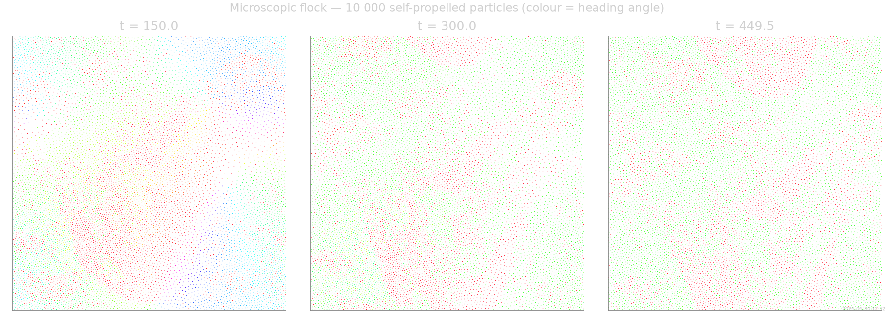
Particle snapshots

Three snapshots inside the banded transient window (frames T_lo, midpoint, T_hi). Heading is HSV-colour-coded; the narrow stripes of common colour, separated by lower-density gaps, are the propagating polar bands characteristic of Toner–Tu / Vicsek flocking.

from SFI.trajectory import TrajectoryCollection

# Wrap the (cached or freshly simulated) microscopic trajectory in a
# collection so the canonical particle/SPDE plotters can read frames
# directly (heading lives in state dimension 2).
coll_micro = TrajectoryCollection.from_arrays(X=X_micro, dt=dt_sim * 10)

snap_idx = [T_lo, (T_lo + T_hi) // 2, T_hi - 1]
fig_snap, axes_snap = plt.subplots(1, 3, figsize=(12, 4.2))
for ax, ti in zip(axes_snap, snap_idx):
    plot_particles(
        coll_micro, t_index=ti, color_dim=2, cmap="hsv",
        vmin=-np.pi, vmax=np.pi, box=box_np, s=2.0,
        alpha=0.85, edgecolors="none", ax=ax,
    )
    ax.set_xlim(0, Lx); ax.set_ylim(0, Ly)
    ax.set_title(f"t = {ti * dt_sim * 10:.1f}")
fig_snap.suptitle(
    "Microscopic flock — 10 000 self-propelled particles (colour = heading angle)",
    fontsize=11,
)
plt.show()

Animated banded flock

Sub-sample particles for clarity, then animate every few frames through the banded window. The HSV colour wheel encodes heading angle, so density stripes of a single colour reveal coherently moving polar bands sweeping across the periodic box.

skip = max(1, (T_hi - T_lo) // 200)

fig_anim, ax_anim = plt.subplots(figsize=(5.4, 5.2))
anim = animate_particles(
    coll_micro, color_dim=2, cmap="hsv", vmin=-np.pi, vmax=np.pi,
    box=box_np, skip=skip, s=2.5, ax=ax_anim,
)
plt.show()

Coarse-graining: particles → continuum fields

At each frame we deposit (1, cosθ_i, sinθ_i) for each particle bilinearly onto a periodic 64×64 grid, then convolve with a wrapped Gaussian of standard deviation σ = 1.5 cells. The result is three smooth fields per cell — the local density ρ and the polar momentum density m = ρ\\langle\\hat e_θ\\rangle.

GRID = (64, 64)
DX_GRID = Lx / GRID[0]
SIGMA_CELLS = 1.5

t0 = time.perf_counter()
fields = coarse_grain_polar(
    jnp.asarray(X_use), box=box, grid_shape=GRID,
    sigma_cells=SIGMA_CELLS, angle_index=2,
)
print(f"Coarse-graining: {fields.shape} in {time.perf_counter() - t0:.1f}s")

# Sanity: integrated density should equal particle count
total_mass = float(fields[0, :, 0].sum() * DX_GRID * DX_GRID)
print(f"∫ρ dA = {total_mass:.1f}  (expected {N_particles})")

# Wrap as a TrajectoryCollection on the grid; dt is the frame stride
# of the saved microscopic trajectory.
from SFI.bases.spde import square_grid_extras
from SFI.trajectory import TrajectoryCollection

DT_FRAME = dt_sim * 10           # save_every=10
box_extras_grid = square_grid_extras(grid_shape=GRID, dx=DX_GRID)

coll_fields = TrajectoryCollection.from_arrays(
    X=np.asarray(fields, dtype=np.float32),
    dt=DT_FRAME,
    extras_global=box_extras_grid,
)
print(f"Field trajectory: ({coll_fields.T}, {coll_fields.N}, {coll_fields.d})")

Coarse-graining: (600, 4096, 3) in 2.3s
∫ρ dA = 10000.0  (expected 10000)
Field trajectory: (600, 4096, 3)

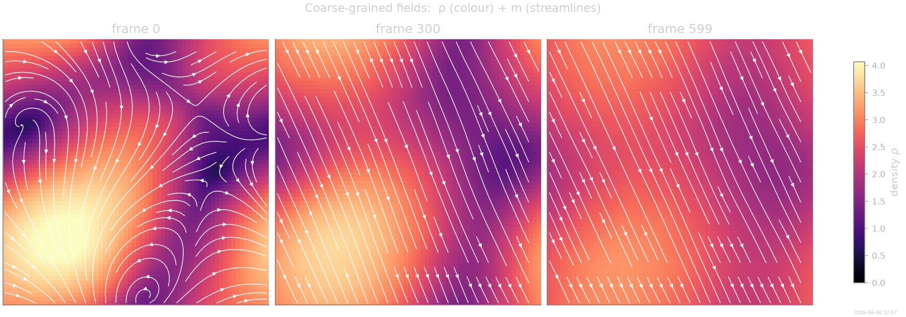
Coarse-grained snapshots

Density ρ (heat map) and polar momentum m (streamlines) at the same physical times as the microscopic snapshots above — minus the burn-in offset.

cg_idx = [0, coll_fields.T // 2, coll_fields.T - 1]
vmax_rho = float(np.percentile(fields[..., 0], 99.5))
stream_kw = dict(density=0.9, color="white", linewidth=0.7, arrowsize=0.7)
fig_cg, axes_cg = plt.subplots(1, 3, figsize=(12, 4.2))
plot_spde_snapshot(
    coll_fields, cg_idx, scalar_channel=0, vector_channels=(1, 2),
    grid_shape=GRID, dx=DX_GRID, render="streamplot",
    vmin=0.0, vmax=vmax_rho, streamplot_kw=stream_kw, axes=axes_cg,
)
for ax, ti in zip(axes_cg, cg_idx):
    ax.set_xlim(0, Lx); ax.set_ylim(0, Ly); ax.set_aspect("equal")
    ax.set_title(f"frame {ti}")
fig_cg.colorbar(axes_cg[0].images[0], ax=axes_cg.tolist(), shrink=0.78,
                label=r"density $\rho$")
fig_cg.suptitle("Coarse-grained fields:  ρ (colour) + m (streamlines)",
                fontsize=11)
plt.show()

Overcomplete SPDE basis: candidate Toner–Tu terms

We assemble ~30 hydrodynamic features with GridLayout:

• ρ-equation (scalar): mass-flux divergence, gradient pressures, and a few pointwise nonlinearities.

• m-equation (vector): linear, cubic, and quintic Landau terms; Frank-elastic ∇²m; pressure-like ∇ρ and ∇|m|²; advective (m·∇)m.

from SFI.statefunc.layout import GridLayout, ScalarSector, VectorSector
from SFI.statefunc.structexpr import StructuredExpr

layout = GridLayout(
    rho=ScalarSector([0]),
    m=VectorSector([1, 2], sdim=2, spatial=True),
    dim=3, ndim=2, bc="pbc",
)
rho = layout.rho
m   = layout.m

# Squared magnitude |m|² (scalar) via einsum contraction
m_sq = StructuredExpr.einsum("i,i->", m, m).with_label("|m|²")

# --- ρ-equation candidates (scalar output per cell) ---
rho_terms = [
    layout.div(m).with_label("∇·m"),
    layout.div(rho * m).with_label("∇·(ρm)"),
    layout.lap(rho),
    (layout.lap(rho * rho)).with_label("∇²ρ²"),
    layout.lap(m_sq).with_label("∇²|m|²"),
    layout.advection_by(m, rho),
    rho.with_label("ρ"),
    (rho * rho).with_label("ρ²"),
    m_sq,
]
rho_basis = rho_terms[0]
for t in rho_terms[1:]:
    rho_basis = rho_basis & t

# --- m-equation candidates (vector output per cell) ---
m_terms = [
    m.with_label("m"),
    (m_sq * m).with_label("|m|²m"),
    ((m_sq * m_sq) * m).with_label("|m|⁴m"),
    layout.lap(m),
    layout.grad(layout.div(m)).with_label("∇(∇·m)"),
    layout.grad(rho).with_label("∇ρ"),
    (layout.grad(rho * rho)).with_label("∇ρ²"),
    layout.grad(m_sq).with_label("∇|m|²"),
    layout.advection_by(m, m),
    (m * layout.div(m)).with_label("m(∇·m)"),
    (rho * m).with_label("ρm"),
]
m_basis = m_terms[0]
for t in m_terms[1:]:
    m_basis = m_basis & t

BASIS = layout.embed(rank=1, rho=rho_basis, m=m_basis)
n_feat = BASIS.n_features
print(f"Overcomplete basis: {n_feat} candidate features "
      f"({len(rho_terms)} for ρ + {len(m_terms)} for m)")

Overcomplete basis: 20 candidate features (9 for ρ + 11 for m)

Linear inference + PASTIS sparsification

from SFI import OverdampedLangevinInference

inf = OverdampedLangevinInference(coll_fields)
inf.compute_diffusion_constant(method="WeakNoise")
inf.infer_force_linear(BASIS, M_mode="Ito")
inf.compute_force_error()

inf.sparsify_force(criterion="PASTIS", p=0.001)
inf.compute_force_error()

k_sel, support_sel, _, coeffs_sel = \
    inf.force_sparsity_result.select_by_ic("PASTIS")

inf.print_report()

  --- StochasticForceInference Report ---
Average diffusion tensor:
 [[ 1.7269813e-05  6.2673080e-06 -1.4041916e-05]
 [ 6.2673080e-06  4.1185002e-04  1.4832322e-04]
 [-1.4041916e-05  1.4832322e-04  1.3275006e-04]]
Measurement noise tensor:
 [[-2.8831907e-06 -8.2338357e-07  9.7881082e-07]
 [-8.2338369e-07  2.5146157e-05  1.8341721e-05]
 [ 9.7881082e-07  1.8341721e-05 -1.5236627e-05]]
Force estimated information: 684290.3125
Force: estimated normalized mean squared error (sampling only): 1.4613569012135748e-05

  Force Coefficient Table
  ─────────────────────────────────────────────────────────────────
  #    Label      Coefficient       Std.Err     SNR  Sig
  ─────────────────────────────────────────────────────────────────
  0    ∇·m       -6.42026e-02   2.15407e-04   298.1  ***
  1    ∇·(ρm)     8.27530e-03   9.87390e-05    83.8  **
  2    ∇²rho      6.85043e-02   8.50566e-04    80.5  **
  3    ∇²ρ²       4.55006e-02   2.37074e-04   191.9  ***
  4    ∇²|m|²    -2.23570e-03   1.50703e-04    14.8  **
  5    (m·∇)rho  -1.19461e-02   1.16922e-04   102.2  ***
  6    ρ          1.30153e-03   1.75887e-05    74.0  **
  7    ρ²        -3.03218e-05   8.01770e-06     3.8  *
  8    |m|²      -4.79972e-04   1.16139e-05    41.3  **
  9    m          3.65620e-03   6.22864e-05    58.7  **
  10   |m|²m     -4.71209e-04   1.20343e-05    39.2  **
  11   |m|⁴m      3.54635e-05   9.29253e-07    38.2  **
  12   ∇²m        3.24034e-01   7.49543e-04   432.3  ***
  13   ∇(∇·m)    -2.26157e-01   1.15357e-03   196.1  ***
  14   ∇ρ        -8.33872e-02   7.32461e-04   113.8  ***
  15   ∇ρ²        9.73189e-03   1.14047e-04    85.3  **
  16   ∇|m|²     -2.23048e-02   1.29393e-04   172.4  ***
  17   (m·∇)m     4.63086e-02   9.44763e-05   490.2  ***
  18   m(∇·m)    -3.17987e-03   1.03356e-04    30.8  **
  19   ρm        -5.32718e-04   4.02552e-05    13.2  **
  ─────────────────────────────────────────────────────────────────
  20/20 basis functions in support, sig: 20* / 19** / 8*** (|SNR| ≥ 2 / 10 / 100)
  (Std.err. reflects sampling error only; discretization bias is not included.)

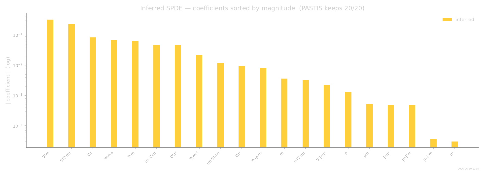
Inferred SPDE: term coefficients

We sort the inferred basis by the magnitude of its coefficient. The few largest terms — Frank elasticity ∇²m, the density Laplacian / divergence-of-flux pair, advective (m·∇)m and the pressure-like ∇ρ — are precisely the canonical Toner–Tu hydrodynamic terms. Sub-dominant nonlinearities span four orders of magnitude below them; they remain statistically significant at this enormous sample size (1050 frames × 4096 cells), so PASTIS keeps them, but they are dynamically negligible.

labels = list(BASIS.labels) if BASIS.labels else [
    f"f{i}" for i in range(n_feat)
]
if len(labels) != n_feat:
    labels = [f"f{i}" for i in range(n_feat)]

# Magnitudes of the PASTIS-selected coefficients, sorted descending on a
# log axis; ``show_pruned`` appends faded zero-bars for the rejected
# candidate terms so the full overcomplete basis stays visible.
fig_bar, ax_bar = plt.subplots(figsize=(13, 4.6))
plot_recovery_bar(
    np.abs(np.asarray(coeffs_sel)), support_sel,
    labels=labels, yscale="log", sort=True, show_pruned=True, ax=ax_bar,
)
ax_bar.set_ylabel(r"$|\,\mathrm{coefficient}\,|$  (log)")
ax_bar.set_title(
    f"Inferred SPDE — coefficients sorted by magnitude  "
    f"(PASTIS keeps {k_sel}/{n_feat})"
)
fig_bar.tight_layout()
plt.show()

examples/gallery/abp_to_spde_demo.py:520: UserWarning: The figure layout has changed to tight
  fig_bar.tight_layout()

Bootstrap: simulate the inferred SPDE

Initialise from random ρ, m fluctuations and integrate the sparse inferred SPDE. If the dynamics are correct, propagating bands should re-emerge spontaneously, just like in the agent-based simulation.

key, bkey = random.split(key)
coll_boot, _ = inf.simulate_bootstrapped_trajectory(
    bkey, oversampling=4, simulate=True,
)
T_boot = coll_boot.T
print(f"Bootstrap SPDE: {T_boot} frames")

Bootstrap SPDE: 600 frames

Bootstrap visualisation

Side-by-side: agent-based bands (left, coarse-grained) vs the bands generated by the inferred SPDE (right) — both at their respective late times.

fig_bs, axes_bs = plt.subplots(1, 2, figsize=(9, 4.6))
vmax_rho = float(np.percentile(fields[..., 0], 99.5))
stream_kw = dict(density=0.9, color="white", linewidth=0.7, arrowsize=0.7)

# Microscopic CG (last frame) vs inferred SPDE (last frame), both as
# ρ heat-map + m streamlines.
plot_spde_snapshot(
    coll_fields, coll_fields.T - 1,
    scalar_channel=0, vector_channels=(1, 2),
    grid_shape=GRID, dx=DX_GRID, render="streamplot",
    vmin=0.0, vmax=vmax_rho, streamplot_kw=stream_kw, axes=axes_bs[0],
)
axes_bs[0].set_title("Agent-based  (coarse-grained)")
axes_bs[0].set_aspect("equal")

plot_spde_snapshot(
    coll_boot, T_boot - 1,
    scalar_channel=0, vector_channels=(1, 2),
    grid_shape=GRID, dx=DX_GRID, render="streamplot",
    vmin=0.0, vmax=vmax_rho, streamplot_kw=stream_kw, axes=axes_bs[1],
)
axes_bs[1].set_title("Inferred SPDE  (PASTIS-sparse)")
axes_bs[1].set_aspect("equal")
fig_bs.suptitle(
    "Bootstrap test — inferred SPDE reproduces the agent-based flock",
    fontsize=11,
)
plt.show()

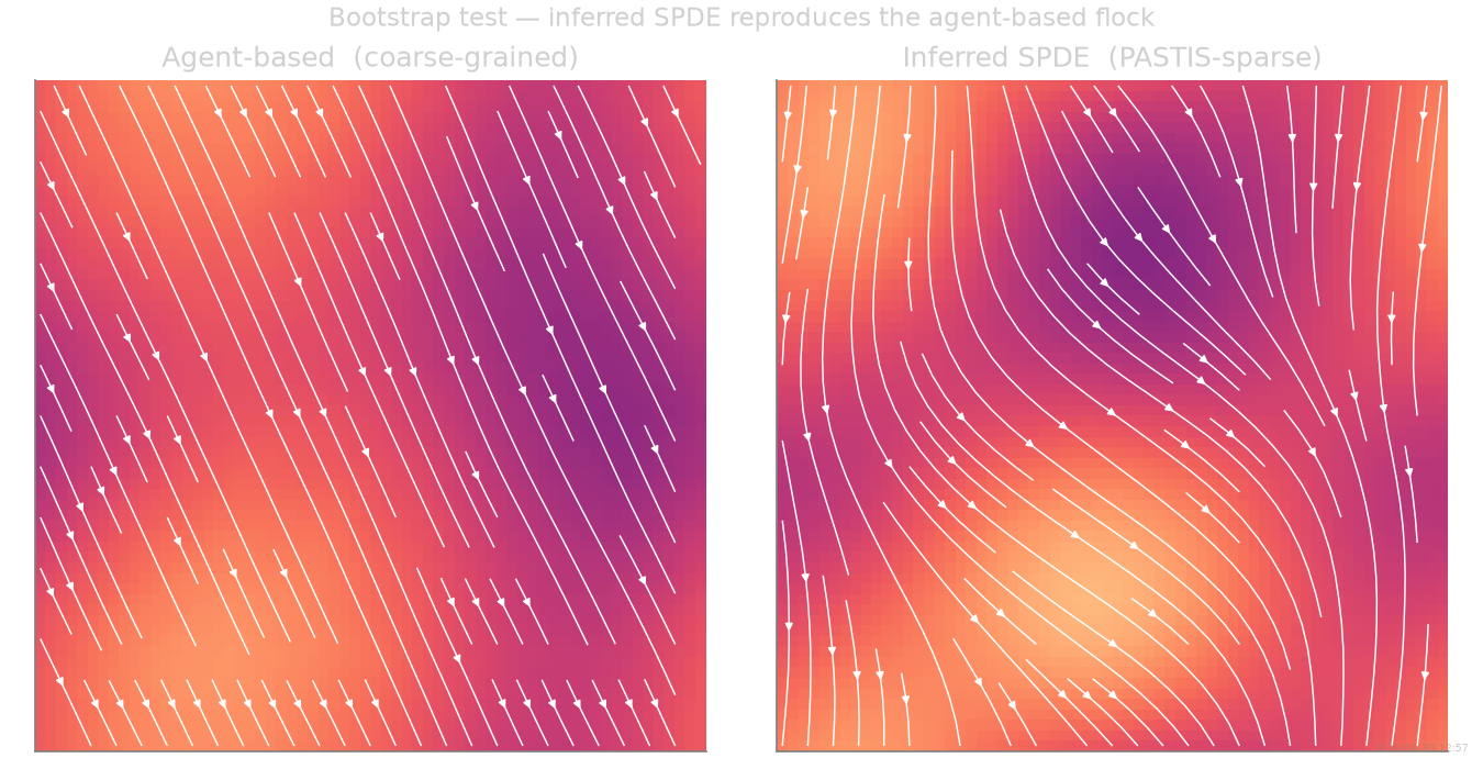
Side-by-side animation: agent-based vs inferred SPDE

The climax: animate the coarse-grained agent-based fields (left) next to the freely-running inferred SPDE (right). Both initialised independently (the SPDE from random fluctuations), and both develop propagating polar bands of comparable amplitude and wavelength — evidence that PASTIS has recovered the dynamics, not just the instantaneous structure.

T_anim = min(coll_fields.T, T_boot)
n_anim_frames = 150
stride = max(1, T_anim // n_anim_frames)
vmax_rho = float(np.percentile(fields[..., 0], 99.5))

anim_dual = animate_spde_comparison(
    coll_fields, coll_boot, grid_shape=GRID,
    field_component=0, skip=stride,
    vmin=0.0, vmax=vmax_rho, interval=60,
    titles=("Agent-based  (coarse-grained)", "Inferred SPDE  (PASTIS-sparse)"),
)
plt.show()

[Generated: 2026-06-30 12:57]

🏷 Tags: synthetic, overdamped, multi-particle, linear, spde, experimental, pastis, interactions