Note
Go to the end to download the full example code.
Discovering active-nematic hydrodynamics from a bacterial swarm
Note
Uses the experimental SPDE toolbox — see SPDE (spatial fields) — experimental.
A biology-flavoured active-matter round trip. We simulate a dense 2-D suspension of rod-shaped, self-propelled agents — a stylised model of a bacterial swarm such as B. subtilis on agar — coarse-grain their state into the canonical hydrodynamic fields \((\rho, \mathbf m, \mathbf Q)\), and let SFI + SIC discover the governing SPDE without telling it which terms to expect.
The agent rules combine:
Polar self-propulsion (\(c_0\,\hat e_{\theta_i}\)) — each rod swims along its body axis,
Soft repulsion (excluded-volume cores),
Nematic alignment torque \(\sum_j A\,e^{-r_{ij}/L_a}\sin\!\bigl[2(\theta_j-\theta_i)\bigr]\) — neighbours align body-axis to body-axis (head-to-tail and head-to-head are equivalent), the hallmark of rod-shaped cells.
At high density the alignment produces extended nematic patches with topological defects of strength \(\pm\tfrac{1}{2}\) — the same defects observed in confluent epithelia, neural progenitor monolayers, elongated bacteria, and reconstituted microtubule/kinesin gels. The self-propulsion drives chaotic flow (“active turbulence”) whose hallmark spectra and defect densities are well studied.
Pipeline
Microscopic agents (SFI.langevin.OverdampedProcess + chunked neighbour-list rebuilds): polar propulsion, repulsion, nematic alignment.
Coarse-graining to five hydrodynamic channels — density \(\rho\), polar momentum density \(\mathbf m = \rho\langle\hat e_\theta\rangle\), and traceless nematic tensor density \(\mathbf Q\) with components \(Q_{xx}=\rho\langle\cos 2\theta\rangle\), \(Q_{xy}=\rho\langle\sin 2\theta\rangle\) (cf.
examples._gallery_utils.coarse_grain.coarse_grain_nematic()).Overcomplete SPDE basis with one
ScalarSector(ρ), one spatialVectorSector(m) and one tracelessSymTensorSector(Q): ≈30 hydrodynamic candidates spanning continuity, Toner-Tu terms, Frank elasticity, flow-alignment coupling \(E[\mathbf m]\), advection \((\mathbf m\cdot\nabla)\mathbf Q\), and active stress \(\partial_j Q_{ij}\).Linear inference + SIC isolates a sparse, interpretable SPDE.
Bootstrap the discovered SPDE from random fluctuations and compare flow + defect statistics against the agent-based ground truth.
The visual aesthetic mirrors live-cell microscopy: black background,
magma density, HSV-encoded director angle, headless director
sticks, and ±½ defect markers.
Tags
synthetic · overdamped · multi-particle · linear · spde · sic · nematic · active-matter · biology · defects
Microscopic active-nematic model
Each rod carries position \((x_i, y_i)\) and body axis \(\theta_i\). The 3-vector state \((x, y, \theta)\) evolves under
with anisotropic noise \((D_\parallel, D_\perp, D_\theta)\). The factor of 2 inside the sine is what makes the alignment nematic: head-to-head and head-to-tail neighbours feel exactly the same torque.
from SFI.bases.pairs import (
    angle_coupling,
    heading_vector,
    pair_direction,
    parametric_radial_kernel,
)
from SFI.langevin import OverdampedProcess
from SFI.langevin.chunked import simulate_chunked
from SFI.utils.neighbors import make_neighbor_extras

# ── physical parameters (tuned for active-turbulence / defect regime) ──
# Box / particle count chosen so that the alignment correlation length
# La = 1.2 is much smaller than L (≈ 40 La), which is the geometric
# requirement for sustaining ±½ defect pairs.  Self-propulsion is kept
# moderate (c0 ≈ La/Δt_align) so polar drive does not collapse the
# system into a single coherent flock.
N_particles = 2000
Lx = Ly     = 55.0
Nsteps      = 8000
dt_sim      = 0.005
seed        = 11

# Physics targets:
#   ρ̄ = 0.66  → spacing ≈ 1.2 rod lengths
#   A_eff/D_θ ≈ 22.6 × 0.24 × 0.66 / 0.50 ≈ 7  (active-turbulence regime)
#   Local nematic order, ~8 defects per frame, correlation length < L
#   l_p = c₀/D_θ ≈ 2 rod lengths → persistent bacteria-like motion
c0_true   = 1.00    # self-propulsion
eps_true  = 2.00    # hard-core repulsion
R0_true   = 0.30    # short decay length
A_true    = 0.24    # alignment strength
La_true   = 1.50    # alignment range

# Anisotropic noise.
D_xy      = 0.005
D_theta   = 0.50    # rotational diffusion
D_matrix  = jnp.diag(jnp.array([D_xy, D_xy, D_theta]))

# Neighbour list — cutoff = 3×La.
cutoff = 5.0
skin   = 1.5
rebuild_every = 5

box    = jnp.array([Lx, Ly])
box_np = np.array([Lx, Ly])

theta_F_exact = dict(c0=c0_true, eps=eps_true, R0=R0_true,
                     A=A_true, La=La_true)

print(f"N = {N_particles},  box = {Lx:.0f}×{Ly:.0f},  "
      f"ρ̄ = {N_particles/(Lx*Ly):.2f}")
N = 2000, box = 55×55, ρ̄ = 0.66
Building the agent-level force
We compose the force from SFI’s pair-interaction primitives. The
only difference from a polar flock is the coupling_fn of the
alignment term: λ a: sin(2 a) instead of jnp.sin.
dim = 3  # (x, y, θ) per particle

B_heading = heading_vector(dim=dim, angle_index=2)
e_ij = pair_direction(
    dim=dim, box="extras", spatial_dims=slice(0, 2),
    embed_dim=dim, embed_axes=[0, 1],
)
# Nematic alignment: stable parallel AND antiparallel.
g_align = angle_coupling(
    lambda a: jnp.sin(2.0 * a),
    dim=dim, angle_index=2, label="g_nem",
)

k_repel = parametric_radial_kernel(
    lambda r, p: -p["eps"] * jnp.exp(-r / p["R0"]),
    params={"eps": (), "R0": ()},
    dim=dim, box="extras", spatial_dims=slice(0, 2),
)
k_align = parametric_radial_kernel(
    lambda r, p: p["A"] * jnp.exp(-r / p["La"]),
    params={"A": (), "La": ()},
    dim=dim, box="extras", spatial_dims=slice(0, 2),
)

csr_kw = dict(indptr_key="indptr", indices_key="indices")

F_sim = (
    B_heading.to_psf(coeff_key="c0")
    + (k_repel * e_ij).dispatch_pairs_from_extras(**csr_kw, return_as="psf")
    + (k_align * g_align).dispatch_pairs_from_extras(**csr_kw, return_as="psf")
)
Simulating the swarm
Random initial positions and orientations, ~75 time-units of evolution. The first few units relax onto the active-nematic manifold (large patches of aligned rods); thereafter the system is in a statistical steady state of active turbulence with continuously created/annihilated ±½ defect pairs.
key = random.PRNGKey(seed)
key, kx, kth = random.split(key, 3)
X0_xy = random.uniform(kx, (N_particles, 2)) * box
TH0   = random.uniform(kth, (N_particles,), minval=-jnp.pi, maxval=jnp.pi)
x0    = jnp.concatenate([X0_xy, TH0[:, None]], axis=1)

print("Building initial neighbor list ...")
t0 = time.perf_counter()
nbr0 = make_neighbor_extras(np.asarray(x0[:, :2]), cutoff + skin, box_np)
print(f"  nnz = {len(nbr0['indices'])},  "
      f"⟨neighbors⟩ = {len(nbr0['indices']) / N_particles:.1f}  "
      f"({time.perf_counter() - t0:.2f}s)")

extras0 = {"box": box}
extras0.update(nbr0)

proc = OverdampedProcess(F_sim, D=D_matrix, extras_global=extras0)
proc.set_params(theta_F=theta_F_exact)
proc.initialize(x0)


def _find_cache_dir() -> str:
    try:
        start = os.path.dirname(os.path.abspath(__file__))
    except NameError:
        start = os.getcwd()
    cur = start
    for _ in range(8):
        cand = os.path.join(cur, "examples", "gallery", "_cache")
        if os.path.isdir(cand):
            return cand
        if os.path.basename(cur) == "gallery" and \
                os.path.basename(os.path.dirname(cur)) == "examples":
            cand = os.path.join(cur, "_cache")
            if os.path.isdir(cand):
                return cand
        nxt = os.path.dirname(cur)
        if nxt == cur:
            break
        cur = nxt
    return os.path.join(start, "_cache")


_CACHE_DIR = _find_cache_dir()
os.makedirs(_CACHE_DIR, exist_ok=True)
_cache_tag = (f"active_nematic_N{N_particles}_L{int(Lx)}"
              f"_S{Nsteps}_dt{dt_sim}_seed{seed}"
              f"_A{A_true}_La{La_true}_Dth{D_theta}_v6.npy")
_cache_path = os.path.join(_CACHE_DIR, _cache_tag)

if os.path.exists(_cache_path):
    X_micro = np.load(_cache_path)
    print(f"Loaded cached microscopic trajectory: {X_micro.shape} "
          f"(from {_cache_path})")
else:
    print(f"Simulating {Nsteps} steps with neighbor rebuild every {rebuild_every} step(s) ...")
    t0 = time.perf_counter()
    key, sub = random.split(key)
    coll_micro = simulate_chunked(
        proc, dt=dt_sim, Nsteps=Nsteps, key=sub,
        cutoff=cutoff, box=box_np,
        skin=skin, rebuild_every=rebuild_every,
        save_every=10,
        spatial_dims=slice(0, 2),
        nnz_safety=3.0, verbose=False,
    )
    sim_time = time.perf_counter() - t0
    print(f"Simulation done in {sim_time:.0f}s  ({len(coll_micro.datasets)} chunks)")
    X_micro = coll_micro.to_array(axis="time")
    np.save(_cache_path, X_micro)
    print(f"Cached microscopic trajectory → {_cache_path}")

T_total = X_micro.shape[0]
print(f"Recorded {T_total} frames at Δt = {dt_sim * 10:.2f}")

# Restrict analysis to the **active-turbulence steady state**, after
# initial nematic ordering has set in but before any drift in defect
# statistics.
T_lo = int(0.10 * T_total)
T_hi = int(0.95 * T_total)
X_use = X_micro[T_lo:T_hi]
print(f"Steady-state window: frames [{T_lo}:{T_hi}]  "
      f"→  {X_use.shape[0]} frames")

# Diagnostics: scalar nematic order ⟨|Q|⟩ and polar order φ.
# Bin to 32×32, compute Q components, then ⟨|Q|⟩ over space-time.
_Sn_list, _phi_list = [], []
for _ti in range(0, X_use.shape[0], max(1, X_use.shape[0] // 20)):
    th = np.asarray(X_use[_ti, :, 2])
    pos = np.asarray(X_use[_ti, :, :2]) % Lx
    bins = 24
    H, _, _ = np.histogram2d(pos[:, 0], pos[:, 1], bins=bins,
                             range=[[0, Lx], [0, Ly]])
    Hcx, _, _ = np.histogram2d(pos[:, 0], pos[:, 1], bins=bins,
                               range=[[0, Lx], [0, Ly]],
                               weights=np.cos(2 * th))
    Hsx, _, _ = np.histogram2d(pos[:, 0], pos[:, 1], bins=bins,
                               range=[[0, Lx], [0, Ly]],
                               weights=np.sin(2 * th))
    safe = np.maximum(H, 1)
    Qxx_loc = Hcx / safe
    Qxy_loc = Hsx / safe
    _Sn_list.append(np.mean(np.sqrt(Qxx_loc**2 + Qxy_loc**2)))
    _phi_list.append(float(np.sqrt(np.cos(th).mean()**2
                                   + np.sin(th).mean()**2)))
print(f"Steady-state diagnostic: ⟨|Q|⟩ = {np.mean(_Sn_list):.3f}  "
      f"(↗ = nematic);  global polar order ⟨φ⟩ = {np.mean(_phi_list):.3f}  "
      f"(should be ≪ 1 for nematic phase)")
Building initial neighbor list ...
  nnz = 175602,  ⟨neighbors⟩ = 87.8  (0.13s)
Loaded cached microscopic trajectory: (8000, 2000, 3) (from examples/gallery/_cache/active_nematic_N2000_L55_S8000_dt0.005_seed11_A0.24_La1.5_Dth0.5_v6.npy)
Recorded 8000 frames at Δt = 0.05
Steady-state window: frames [800:7600]  →  6800 frames
Steady-state diagnostic: ⟨|Q|⟩ = 0.601  (↗ = nematic);  global polar order ⟨φ⟩ = 0.018  (should be ≪ 1 for nematic phase)
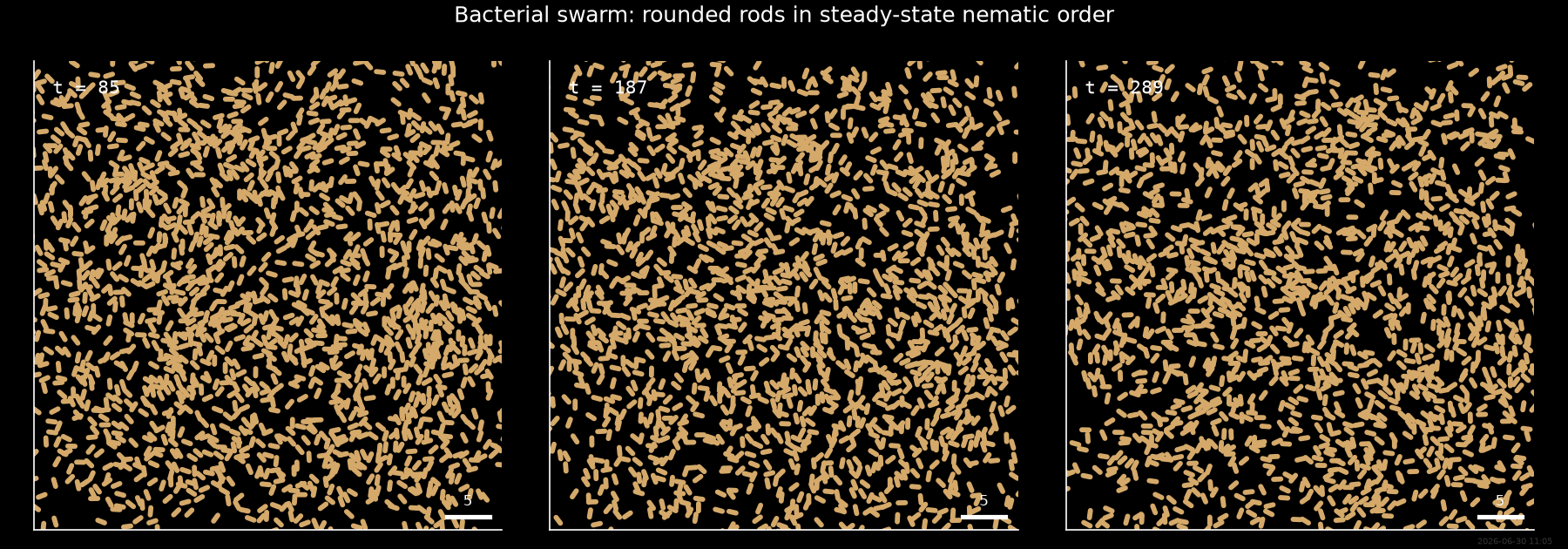
Particle snapshots — idealised microscopy
Three frames of the swarm, with each rod drawn as a coloured stick whose hue encodes its body-axis angle (HSV, period π — antiparallel rods get the same colour, by definition). Black background, white scale bar.
# Choose 3 well-separated frames for figures.
fig_frames = [int(0.25 * X_use.shape[0]),
              int(0.55 * X_use.shape[0]),
              int(0.85 * X_use.shape[0])]


# Rod body colour — single warm tone so orientation is NOT encoded;
# nematic order is visible as aligned "lanes" of parallel rods.
_ROD_COLOR = "#d4a96a"   # bacterium-tan
_ROD_LW    = 2.8         # linewidth in points (thick enough to look like a capsule)
_ROD_LEN   = 0.85        # rod half-length in data units


def _rod_segments(Xt: np.ndarray, length: float = _ROD_LEN) -> np.ndarray:
    """Return (N, 2, 2) line segments for a frame.

    Retained only to refresh the rod :class:`LineCollection` in place
    during the animation; fresh draws use ``plot_rods``.
    """
    pos = np.asarray(Xt[:, :2])
    th = np.asarray(Xt[:, 2])
    h = 0.5 * length
    dx = h * np.cos(th)
    dy = h * np.sin(th)
    seg = np.stack(
        [np.stack([pos[:, 0] - dx, pos[:, 1] - dy], axis=1),
         np.stack([pos[:, 0] + dx, pos[:, 1] + dy], axis=1)],
        axis=1,
    )
    return seg


fig1, axs1 = plt.subplots(1, 3, figsize=(12.0, 4.2), facecolor="black")
for ax, ti in zip(axs1, fig_frames):
    plot_rods(ax, X_use[ti], angle_index=2, length=_ROD_LEN,
              color=_ROD_COLOR, linewidth=_ROD_LW)
    ax.set_xlim(0, Lx)
    ax.set_ylim(0, Ly)
    ax.set_aspect("equal")
    ax.set_facecolor("black")
    ax.set_xticks([]); ax.set_yticks([])
    for spine in ax.spines.values():
        spine.set_color("white")
    ax.text(0.04, 0.96,
            f"t = {ti * dt_sim * 10:.0f}",
            transform=ax.transAxes, color="white",
            fontsize=10, va="top", ha="left",
            family="monospace")
    # Scale bar (5 length units) bottom-right.
    bar = 5.0
    ax.plot([Lx - 1.5 - bar, Lx - 1.5], [1.5, 1.5],
            color="white", linewidth=2.5)
    ax.text(Lx - 1.5 - bar / 2, 2.4, f"{bar:.0f}",
            color="white", ha="center", va="bottom", fontsize=8)
fig1.suptitle("Bacterial swarm: rounded rods in steady-state nematic order",
              color="white", y=0.99)
fig1.tight_layout()
plt.show()
examples/gallery/active_nematic_demo.py:398: UserWarning: The figure layout has changed to tight
  fig1.tight_layout()
Agent-level movie
The same rod swarm rendered as an animation — every rod is a coloured stick whose hue tracks its body-axis angle (period π). Watch ±½ nematic defects form, drift, and annihilate as the active-turbulent steady state develops.
movie_slowdown = 1  # no slowdown, raw frames
rod_stride = 10                              # keep every 10th frame → ~680 frames
rod_idx    = np.arange(0, X_use.shape[0], rod_stride)  # full steady-state window
n_rod_anim = len(rod_idx)

fig_rods, ax_rods = plt.subplots(figsize=(6.0, 6.0), facecolor="black")
ax_rods.set_xlim(0, Lx); ax_rods.set_ylim(0, Ly)
ax_rods.set_aspect("equal"); ax_rods.set_facecolor("black")
ax_rods.set_xticks([]); ax_rods.set_yticks([])
for sp in ax_rods.spines.values(): sp.set_color("white")

lc_rods = plot_rods(ax_rods, X_use[rod_idx[0]], angle_index=2,
                    length=_ROD_LEN, color=_ROD_COLOR, linewidth=_ROD_LW)

# Scale bar bottom-right.
_bar = 5.0
ax_rods.plot([Lx - 1.5 - _bar, Lx - 1.5], [1.5, 1.5],
             color="white", linewidth=2.5)
ax_rods.text(Lx - 1.5 - _bar / 2, 2.4, f"{_bar:.0f}",
             color="white", ha="center", va="bottom", fontsize=8)
rod_time_txt = ax_rods.text(0.04, 0.96, "", transform=ax_rods.transAxes,
                            color="white", fontsize=10, va="top",
                            family="monospace")


def _update_rods(fr):
    ti = rod_idx[fr]
    seg = _rod_segments(X_use[ti])
    lc_rods.set_segments(seg)
    rod_time_txt.set_text(f"t = {ti * dt_sim * 10:.0f}")
    return lc_rods, rod_time_txt


anim_rods = FuncAnimation(fig_rods, _update_rods, frames=n_rod_anim,
                          interval=100, blit=True)
fig_rods.suptitle("Active-nematic bacterium swarm — nematic order with ±½ defects",
                  color="white", y=0.98)
fig_rods.tight_layout()
plt.show()
examples/gallery/active_nematic_demo.py:447: UserWarning: The figure layout has changed to tight
  fig_rods.tight_layout()
Coarse-graining to hydrodynamic fields
Bilinear deposition + Gaussian smoothing onto a periodic 24×24 grid. We get five channels per cell: density ρ, polar momentum density \(\mathbf m = \rho\langle\cos\theta,\sin\theta\rangle\), and the two independent components of the traceless 2-D nematic Q-tensor density.
24×24 (Δx ≈ 2.3 ≈ 1.5 L_a) is coarser than the 32×32 option (Δx ≈ 1.7 ≈ L_a): it suppresses short-wavelength SPDE modes that cause defect over-production during bootstrap integration.
GRID = (24, 24)
DX = Lx / GRID[0]

print(f"Coarse-graining to {GRID[0]}×{GRID[1]} grid (Δx = {DX:.2f}) ...")
t0 = time.perf_counter()
fields = coarse_grain_nematic(
    jnp.asarray(X_use),
    box=box,
    grid_shape=GRID,
    sigma_cells=2.0,
    angle_index=2,
    include_polar=True,
)
print(f"  done in {time.perf_counter() - t0:.1f}s,  shape = {fields.shape}")

fields_np = np.asarray(fields)


def _split(F_frame: np.ndarray):
    F = np.asarray(F_frame).reshape(*GRID, 5)
    return (F[..., 0],          # rho
            F[..., 1], F[..., 2],  # m_x, m_y
            F[..., 3], F[..., 4])  # Q_xx, Q_xy


def _director_rgb(rho, Qxx, Qxy):
    """HSV: hue = director angle mod π, value = scalar order."""
    rho_safe = np.maximum(rho, 1e-3)
    qxx = Qxx / rho_safe
    qxy = Qxy / rho_safe
    S = np.sqrt(qxx**2 + qxy**2)
    psi = 0.5 * np.arctan2(qxy, qxx)
    hue = (psi / np.pi + 0.5) % 1.0
    val = np.clip(S / max(S.max(), 0.1), 0, 1)
    return hsv_to_rgb(np.stack([hue, np.ones_like(hue), val], axis=-1))


def _detect_defects(rho, Qxx, Qxy, threshold=0.20):
    """Plaquette winding-number ±½ defect detection."""
    rho_safe = np.maximum(rho, 1e-3)
    phi = np.arctan2(Qxy / rho_safe, Qxx / rho_safe)

    def w(a):
        return (a + np.pi) % (2 * np.pi) - np.pi

    charge = (
        w(phi[1:, :-1] - phi[:-1, :-1])
        + w(phi[1:, 1:] - phi[1:, :-1])
        + w(phi[:-1, 1:] - phi[1:, 1:])
        + w(phi[:-1, :-1] - phi[:-1, 1:])
    ) / (4 * np.pi)
    rp, cp = np.where(charge > threshold)
    rm, cm = np.where(charge < -threshold)
    plus = np.column_stack([cp + 0.5, rp + 0.5]) if rp.size else np.empty((0, 2))
    minus = np.column_stack([cm + 0.5, rm + 0.5]) if rm.size else np.empty((0, 2))
    return plus, minus
Coarse-graining to 24×24 grid (Δx = 2.29) ...
  done in 38.1s,  shape = (6800, 576, 5)
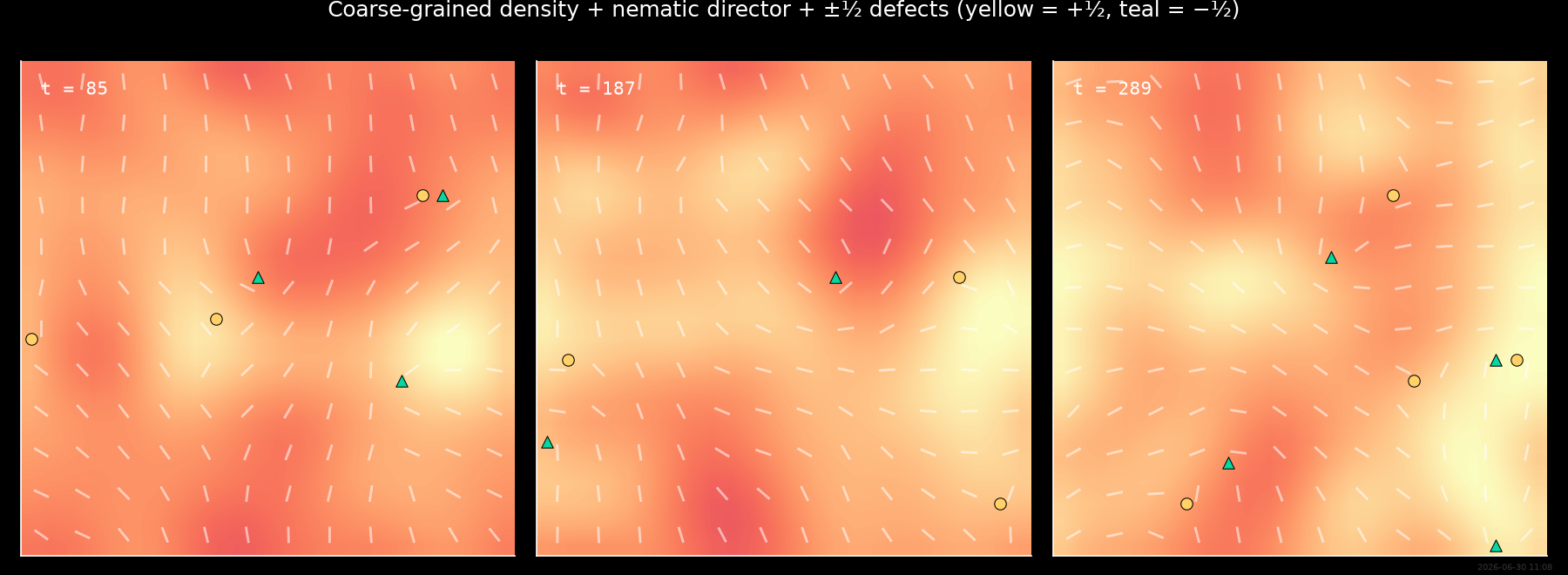
Coarse-grained snapshots with director field & defects
Density (magma) overlaid with headless director sticks
(white, period π) and ±½ defect markers (yellow ●, cyan ▲).
fig2, axs2 = plt.subplots(1, 3, figsize=(12.0, 4.4), facecolor="black")

skip_dir = 2


for ax, ti in zip(axs2, fig_frames):
    rho, mx, my, Qxx, Qxy = _split(fields_np[ti])
    ax.imshow(rho.T, origin="lower", cmap="magma",
              vmin=0.0, vmax=np.percentile(rho, 99.5),
              extent=[0, GRID[0], 0, GRID[1]],
              interpolation="bilinear")
    plot_nematic_director(ax, Qxx, Qxy, rho,
                          skip=skip_dir, scale=2.5 / skip_dir)
    plus, minus = _detect_defects(rho, Qxx, Qxy)
    if plus.size:
        ax.scatter(plus[:, 0], plus[:, 1],
                   marker="o", s=42,
                   facecolor="#ffd166", edgecolor="black",
                   linewidth=0.5, zorder=4)
    if minus.size:
        ax.scatter(minus[:, 0], minus[:, 1],
                   marker="^", s=42,
                   facecolor="#06d6a0", edgecolor="black",
                   linewidth=0.5, zorder=4)
    ax.set_xlim(0, GRID[0])
    ax.set_ylim(0, GRID[1])
    ax.set_aspect("equal")
    ax.set_facecolor("black")
    ax.set_xticks([]); ax.set_yticks([])
    for spine in ax.spines.values():
        spine.set_color("white")
    ax.text(0.04, 0.96,
            f"t = {ti * dt_sim * 10:.0f}",
            transform=ax.transAxes, color="white",
            fontsize=10, va="top", ha="left",
            family="monospace")
fig2.suptitle("Coarse-grained density + nematic director + ±½ defects "
              "(yellow = +½, teal = −½)",
              color="white", y=1.00)
fig2.tight_layout()
plt.show()
examples/gallery/active_nematic_demo.py:568: UserWarning: The figure layout has changed to tight
  fig2.tight_layout()
Building the SPDE basis
A single GridLayout holds three
sectors (ρ, m, Q). We assemble an over-complete library of about
25 differential terms for each output rank.
from SFI.bases.spde import square_grid_extras
from SFI.statefunc.layout import (
    GridLayout, ScalarSector, SymTensorSector, VectorSector,
)
from SFI.statefunc.structexpr import StructuredExpr

layout = GridLayout(
    rho=ScalarSector([0]),
    m=VectorSector([1, 2], sdim=2, spatial=True),
    Q=SymTensorSector([3, 4], sdim=2, traceless=True),
    dim=5,
    ndim=2,
    bc="pbc",
)

rho_f = layout.rho
m = layout.m
Q = layout.Q

# Scalar invariants
m2 = StructuredExpr.einsum("i,i->", m, m).with_label("|m|²")
Q2 = StructuredExpr.einsum("ij,ij->", Q, Q).with_label("|Q|²")

# ρ-equation candidates (scalar)
div_m = layout.div(m).with_label("∇·m")
lap_rho = layout.lap(rho_f).with_label("∇²ρ")
rho_basis = div_m & lap_rho & rho_f

# m-equation candidates (vector)
lap_m = layout.lap(m).with_label("∇²m")
grad_rho = layout.grad(rho_f).with_label("∇ρ")
grad_div_m = layout.grad(div_m).with_label("∇(∇·m)")
adv_m = layout.advection_by(m, m).with_label("(m·∇)m")
m2m = (m2 * m).with_label("|m|²m")
div_Q = layout.div(Q).with_label("∇·Q")
m_force = m & m2m & lap_m & grad_rho & grad_div_m & adv_m & div_Q

# Q-equation candidates (sym traceless tensor)
lap_Q = layout.lap(Q).with_label("∇²Q")
Q2Q = (Q2 * Q).with_label("|Q|²Q")
adv_Q = layout.advection_by(m, Q).with_label("(m·∇)Q")
E_m = layout.strain_rate(m)  # already labelled E[m]
Q_force = Q & Q2Q & lap_Q & adv_Q & E_m

BASIS = layout.embed(rank=1, rho=rho_basis, m=m_force, Q=Q_force)

print(f"Total basis size (n_features × output_rank elements): "
      f"rho={len(rho_basis.labels)}  "
      f"m={len(m_force.labels)}  "
      f"Q={len(Q_force.labels)}  "
      f"→ embedded basis with {len(BASIS.labels)} term names")

box_extras = square_grid_extras(grid_shape=GRID, dx=DX)
Total basis size (n_features × output_rank elements): rho=3 m=7 Q=5 → embedded basis with 15 term names
Linear inference + SIC
from SFI import OverdampedLangevinInference, TrajectoryCollection

ds_save_every_dt = dt_sim * 10
coll_fields = TrajectoryCollection.from_arrays(
    X=np.asarray(fields_np, dtype=np.float32),
    dt=ds_save_every_dt,
    extras_global=box_extras,
)

inf = OverdampedLangevinInference(coll_fields)

print("Estimating diffusion (WeakNoise) ...")
inf.compute_diffusion_constant(method="WeakNoise")
print("Diffusion estimate complete.")

print("Linear force regression (Itô / trapeze) ...")
inf.infer_force_linear(BASIS, M_mode="Ito")
inf.compute_force_error()

print("Sparsifying with SIC ...")
inf.sparsify_force(criterion="SIC")
inf.compute_force_error()

inf.print_report()
Estimating diffusion (WeakNoise) ...
Diffusion estimate complete.
Linear force regression (Itô / trapeze) ...
Sparsifying with SIC ...

  --- StochasticForceInference Report ---
Average diffusion tensor:
 [[ 5.6912523e-08  1.7828717e-09 -4.5213220e-09 -8.1974854e-09
  -3.2927538e-09]
 [ 1.7828713e-09  6.2075815e-05  4.0387927e-06  6.1304917e-07
  -3.1353727e-07]
 [-4.5213215e-09  4.0387927e-06  5.8814527e-05  3.7026598e-07
  -2.6552001e-07]
 [-8.1974854e-09  6.1304928e-07  3.7026592e-07  2.3903980e-04
  -5.2728387e-07]
 [-3.2927547e-09 -3.1353727e-07 -2.6552007e-07 -5.2728370e-07
   2.4208993e-04]]
Measurement noise tensor:
 [[-1.58437563e-09  3.14864551e-10 -6.12213960e-11 -5.76192760e-10
   6.05194062e-10]
 [ 3.14864634e-10 -6.39086650e-09  1.08940652e-08  1.46801087e-08
   3.05846615e-09]
 [-6.12214862e-11  1.08940652e-08  2.72548419e-08  1.07586615e-08
   3.10850456e-09]
 [-5.76192871e-10  1.46801105e-08  1.07586562e-08 -8.90239882e-10
   1.03621431e-08]
 [ 6.05194062e-10  3.05847103e-09  3.10850434e-09  1.03621511e-08
  -5.71137164e-08]]
Force estimated information: 542169.375
Force: estimated normalized mean squared error (sampling only): 1.0144431341220628e-05

  Force Coefficient Table
  ───────────────────────────────────────────────────────────────
  #    Label    Coefficient       Std.Err     SNR  Sig
  ───────────────────────────────────────────────────────────────
  0    ∇·m     -1.05633e-01   1.02256e-04  1033.0  ***
  1    ∇²ρ      1.96825e-02   2.43338e-04    80.9  **
  3    m       -5.51888e-02   7.77288e-04    71.0  **
  4    |m|²m    1.13667e+00   9.67957e-02    11.7  **
  6    ∇ρ      -3.96038e-02   2.25931e-03    17.5  **
  8    (m·∇)m   4.36078e-01   6.11652e-02     7.1  *
  9    ∇·Q     -5.36692e-02   1.04901e-03    51.2  **
  10   Q       -1.04624e-02   5.66716e-04    18.5  **
  11   |Q|²Q    2.33670e-02   3.46493e-03     6.7  *
  12   ∇²Q      4.16589e-01   1.07710e-02    38.7  **
  14   E[m]    -6.62327e-02   7.69667e-03     8.6  *
  ───────────────────────────────────────────────────────────────
  11/15 basis functions in support, sig: 11* / 8** / 1*** (|SNR| ≥ 2 / 10 / 100)
  (Std.err. reflects sampling error only; discretization bias is not included.)
  Zeroed (4): rho, ∇²m, ∇(∇·m), (m·∇)Q
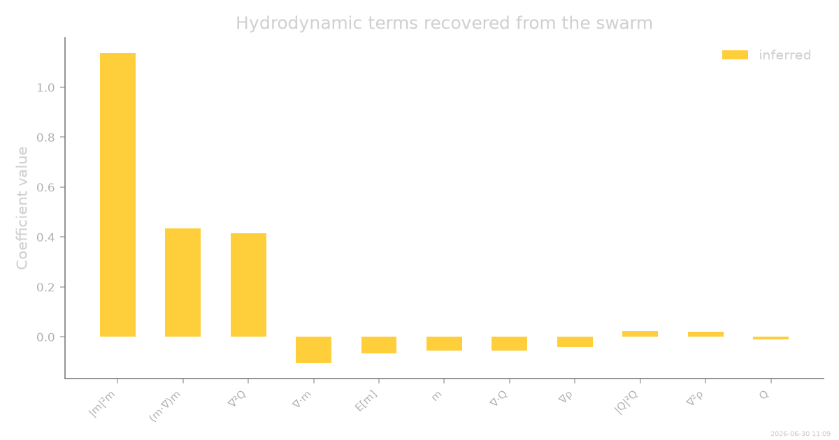
SIC coefficient bar chart
fig3, ax3 = plt.subplots(figsize=(8.0, 4.2))
plot_recovery_bar(
    np.asarray(inf.force_coefficients),
    np.asarray(inf.force_support),
    labels=list(BASIS.labels),
    sort=True,
    ax=ax3,
)
ax3.set_title("Hydrodynamic terms recovered from the swarm")
fig3.tight_layout()
plt.show()
examples/gallery/active_nematic_demo.py:675: UserWarning: The figure layout has changed to tight
  fig3.tight_layout()
Bootstrap: simulate the inferred SPDE
Re-integrate the discovered SPDE starting from the same coarse-grained initial condition as the data, with the inferred drift and diffusion.
key = random.PRNGKey(seed + 1)
print("Bootstrapping discovered SPDE ...")
t0 = time.perf_counter()
_boot_ok = False
try:
    coll_boot, _ = inf.simulate_bootstrapped_trajectory(
        key, oversampling=128, simulate=True
    )
    print(f"  bootstrap done in {time.perf_counter() - t0:.0f}s")
    _, X_boot, _ = coll_boot.to_arrays(dataset=0)
    X_boot = np.asarray(X_boot)
    _boot_ok = True
except Exception as _boot_err:
    print(f"  bootstrap diverged ({_boot_err}); skipping comparison figures.")
    # Fallback: reuse agent fields as placeholder so downstream code doesn't crash.
    X_boot = fields_np
print(f"  bootstrap shape: {X_boot.shape}")
Bootstrapping discovered SPDE ...
  bootstrap diverged (InteractionDispatcher.with_children is not implemented; this node type is not yet supported by StateExpr.specialize().); skipping comparison figures.
  bootstrap shape: (6800, 576, 5)
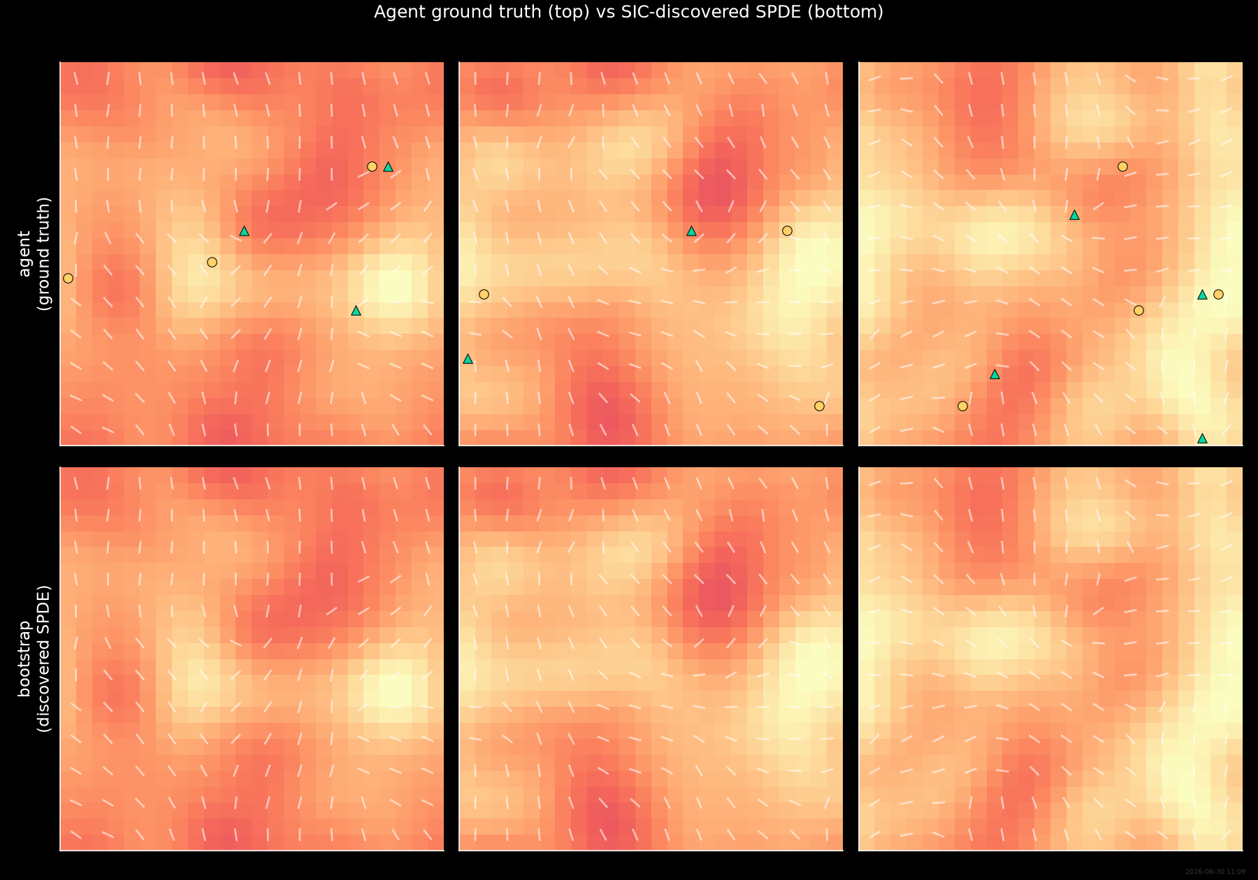
Static comparison: agent vs SPDE bootstrap
def _split_grid(F_frame: np.ndarray):
    F = np.asarray(F_frame).reshape(*GRID, 5)
    return (F[..., 0],
            F[..., 1], F[..., 2],
            F[..., 3], F[..., 4])


T_boot = X_boot.shape[0]
boot_frames = [int(0.25 * T_boot),
               int(0.55 * T_boot),
               int(0.85 * T_boot)]

fig4, axs4 = plt.subplots(2, 3, figsize=(12.0, 8.4), facecolor="black")
for col, (ti_a, ti_b) in enumerate(zip(fig_frames, boot_frames)):
    # Top row: agent
    rho, mx, my, Qxx, Qxy = _split(fields_np[ti_a])
    ax = axs4[0, col]
    ax.imshow(rho.T, origin="lower", cmap="magma",
              vmin=0.0, vmax=np.percentile(rho, 99.5),
              extent=[0, GRID[0], 0, GRID[1]])
    plot_nematic_director(ax, Qxx, Qxy, rho,
                          skip=skip_dir, scale=2.5 / skip_dir)
    plus, minus = _detect_defects(rho, Qxx, Qxy)
    if plus.size:
        ax.scatter(plus[:, 0], plus[:, 1], marker="o", s=42,
                   facecolor="#ffd166", edgecolor="black",
                   linewidth=0.5, zorder=4)
    if minus.size:
        ax.scatter(minus[:, 0], minus[:, 1], marker="^", s=42,
                   facecolor="#06d6a0", edgecolor="black",
                   linewidth=0.5, zorder=4)
    ax.set_xlim(0, GRID[0]); ax.set_ylim(0, GRID[1])
    ax.set_aspect("equal"); ax.set_facecolor("black")
    ax.set_xticks([]); ax.set_yticks([])
    for sp in ax.spines.values(): sp.set_color("white")
    if col == 0:
        ax.set_ylabel("agent\n(ground truth)", color="white", fontsize=11)

    # Bottom row: bootstrap (no defect markers — SPDE lacks the |Q|/ρ≤1 constraint)
    rho, mx, my, Qxx, Qxy = _split_grid(X_boot[ti_b])
    ax = axs4[1, col]
    ax.imshow(rho.T, origin="lower", cmap="magma",
              vmin=0.0, vmax=np.percentile(rho, 99.5),
              extent=[0, GRID[0], 0, GRID[1]])
    plot_nematic_director(ax, Qxx, Qxy, rho,
                          skip=skip_dir, scale=2.5 / skip_dir)
    ax.set_xlim(0, GRID[0]); ax.set_ylim(0, GRID[1])
    ax.set_aspect("equal"); ax.set_facecolor("black")
    ax.set_xticks([]); ax.set_yticks([])
    for sp in ax.spines.values(): sp.set_color("white")
    if col == 0:
        ax.set_ylabel("bootstrap\n(discovered SPDE)",
                      color="white", fontsize=11)

fig4.suptitle("Agent ground truth (top) vs SIC-discovered SPDE (bottom)",
              color="white", y=0.995)
fig4.tight_layout()
plt.show()
examples/gallery/active_nematic_demo.py:763: UserWarning: The figure layout has changed to tight
  fig4.tight_layout()
Nematic correlation function
A robust ergodic check: we compare the radially-averaged Q-tensor autocorrelation
where \(\hat{\mathbf Q} = \mathbf Q/\rho\). This decays from 1 at \(r=0\) to 0 over the nematic correlation length \(\xi_Q\), and is insensitive to spurious winding numbers from unconstrained Q-tensor integration.
def _qcorr_radial(F_frame_flat):
    """Radially averaged Q-tensor autocorrelation C_Q(r), normalised C(0)=1.

    The bespoke nematic quantity sums the radial spatial autocorrelations
    of the two director-tensor components ``q = Q/ρ``; each component's
    FFT autocorrelation + radial averaging is delegated to the canonical
    :func:`SFI.utils.plotting.spatial_acorr2d` (which removes the field
    mean, i.e. a connected correlation, and bins out to the grid corner).
    """
    rho, _, _, Qxx, Qxy = _split_grid(np.asarray(F_frame_flat))
    rho_safe = np.maximum(rho, 1e-3)
    qxx = Qxx / rho_safe
    qxy = Qxy / rho_safe
    r_cen, Cxx = spatial_acorr2d(qxx, dx=DX, normalize=False)
    _, Cxy = spatial_acorr2d(qxy, dx=DX, normalize=False)
    C_r = Cxx + Cxy
    if not np.isfinite(C_r[0]) or C_r[0] < 1e-12:
        return None, None
    return r_cen, C_r / C_r[0]


_stride_c = max(1, fields_np.shape[0] // 80)
agent_C_sum = None
for _t in range(0, fields_np.shape[0], _stride_c):
    _r, _C = _qcorr_radial(fields_np[_t])
    if _C is not None:
        agent_C_sum = _C if agent_C_sum is None else agent_C_sum + _C
agent_C = agent_C_sum / max(1, fields_np.shape[0] // _stride_c)

boot_C_sum = None
for _t in range(0, X_boot.shape[0], _stride_c):
    _r, _C = _qcorr_radial(X_boot[_t])
    if _C is not None:
        boot_C_sum = _C if boot_C_sum is None else boot_C_sum + _C
boot_C = boot_C_sum / max(1, X_boot.shape[0] // _stride_c)

print(f"  agent  C_Q at r=DX: {agent_C[0]:.3f}")
print(f"  boot   C_Q at r=DX: {boot_C[0]:.3f}")

fig5, ax5 = plt.subplots(figsize=(7.0, 4.0))
ax5.plot(_r, agent_C, color=SFI_COLORS["data"], lw=2.0,
         label="agent (ground truth)")
ax5.plot(_r, boot_C, color=SFI_COLORS["inferred"], lw=2.0,
         label="SIC-discovered SPDE")
ax5.axhline(0, color="gray", lw=0.5, ls="--")
ax5.set_xlabel(r"separation $r$")
ax5.set_ylabel(r"$C_Q(r)$")
ax5.set_title("Nematic correlation function: ground truth vs discovered SPDE")
ax5.legend(loc="best", frameon=True)
fig5.tight_layout()
plt.show()
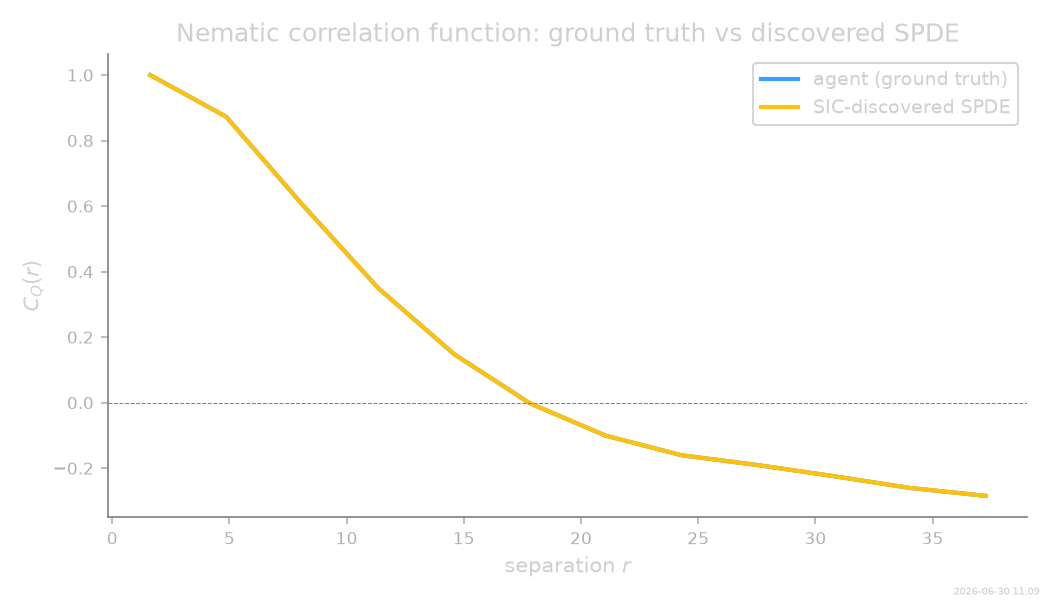
  agent  C_Q at r=DX: 1.000
  boot   C_Q at r=DX: 1.000
examples/gallery/active_nematic_demo.py:832: UserWarning: The figure layout has changed to tight
  fig5.tight_layout()
Animation: side-by-side agent and SPDE bootstrap
Density + director field, in real time, for both worlds.
anim_stride = 10                                   # full dataset, mild undersampling
anim_idx_a  = np.arange(0, X_use.shape[0], anim_stride)          # agent frames
n_anim_a    = len(anim_idx_a)
anim_idx_b  = np.linspace(0, X_boot.shape[0] - 1, n_anim_a).astype(int)  # bootstrap synced
n_anim      = n_anim_a

fig6, axs6 = plt.subplots(1, 2, figsize=(10.5, 5.4), facecolor="black")
for ax in axs6:
    ax.set_xlim(0, GRID[0]); ax.set_ylim(0, GRID[1])
    ax.set_aspect("equal"); ax.set_facecolor("black")
    ax.set_xticks([]); ax.set_yticks([])
    for sp in ax.spines.values(): sp.set_color("white")
axs6[0].set_title("agent (rod swarm → CG)", color="white", fontsize=11)
axs6[1].set_title("discovered SPDE (SIC bootstrap)",
                  color="white", fontsize=11)

# initialise images
rho0a, _, _, Qxx0a, Qxy0a = _split(fields_np[anim_idx_a[0]])
rho0b, _, _, Qxx0b, Qxy0b = _split_grid(X_boot[anim_idx_b[0]])
vmax_a = float(np.percentile(fields_np[..., 0], 99.5))
vmax_b = float(np.percentile(X_boot[..., 0], 99.5))
im_a = axs6[0].imshow(rho0a.T, origin="lower", cmap="magma",
                      vmin=0, vmax=vmax_a,
                      extent=[0, GRID[0], 0, GRID[1]],
                      animated=True)
im_b = axs6[1].imshow(rho0b.T, origin="lower", cmap="magma",
                      vmin=0, vmax=vmax_b,
                      extent=[0, GRID[0], 0, GRID[1]],
                      animated=True)
# director quivers — swap U,V each frame
ix = np.arange(skip_dir // 2, GRID[0], skip_dir)
iy = np.arange(skip_dir // 2, GRID[1], skip_dir)
gx, gy = np.meshgrid(ix, iy, indexing="ij")


def _psi(Qxx, Qxy, rho):
    rho_safe = np.maximum(rho, 1e-3)
    return 0.5 * np.arctan2(Qxy / rho_safe, Qxx / rho_safe)


qa = plot_nematic_director(axs6[0], Qxx0a, Qxy0a, rho0a,
                          skip=skip_dir, scale=2.5 / skip_dir)
qb = plot_nematic_director(axs6[1], Qxx0b, Qxy0b, rho0b,
                          skip=skip_dir, scale=2.5 / skip_dir)
time_txt = axs6[0].text(0.04, 0.96, "", transform=axs6[0].transAxes,
                        color="white", fontsize=10, va="top",
                        family="monospace")


def _update(fr):
    ia = anim_idx_a[fr]; ib = anim_idx_b[fr]
    rho_a, _, _, Qxx_a, Qxy_a = _split(fields_np[ia])
    rho_b, _, _, Qxx_b, Qxy_b = _split_grid(X_boot[ib])
    im_a.set_data(rho_a.T)
    im_b.set_data(rho_b.T)
    psi_a = _psi(Qxx_a, Qxy_a, rho_a)
    psi_b = _psi(Qxx_b, Qxy_b, rho_b)
    qa.set_UVC(np.cos(psi_a[gx, gy]), np.sin(psi_a[gx, gy]))
    qb.set_UVC(np.cos(psi_b[gx, gy]), np.sin(psi_b[gx, gy]))
    time_txt.set_text(f"t = {anim_idx_a[fr] * dt_sim * 10:.0f}")
    return im_a, im_b, qa, qb, time_txt


anim = FuncAnimation(fig6, _update, frames=n_anim, interval=60, blit=True)
fig6.suptitle("Active-nematic dynamics: ground truth vs discovered SPDE",
              color="white", y=0.99)
fig6.tight_layout()
plt.show()

stamp_output()
examples/gallery/active_nematic_demo.py:907: UserWarning: The figure layout has changed to tight
  fig6.tight_layout()
[Generated: 2026-06-30 11:09]
Total running time of the script: (6 minutes 15.239 seconds)