Getting started: end-to-end inference (Ornstein–Uhlenbeck)

This is the recommended starting point for new users: a complete, runnable Stochastic Force Inference (SFI) workflow on the simplest non-trivial system. Every step below is executed when the documentation is built, so the numbers and figures on this page are real output.

We work with a one-dimensional Ornstein–Uhlenbeck (OU) process — a particle in a harmonic trap. Its motion obeys the simplest overdamped Langevin equation,

\[\mathrm{d}x = \underbrace{-k\,x}_{F(x)}\,\mathrm{d}t + \sqrt{2D}\;\mathrm{d}W ,\]

a linear restoring force \(F(x) = -k\,x\) that pulls the particle back toward the origin, plus white noise whose strength is set by the diffusion constant \(D\). Because the force is linear and the noise constant, we know the exact answer in advance — which makes OU the ideal system for watching the method work.

Across this page we will:

1. simulate a trajectory from a known model;

2. estimate the diffusion constant and infer the force;

3. let SFI select the minimal model out of a deliberately over-complete basis;

4. validate the fit with residual diagnostics and a bootstrapped trajectory;

5. save the result to disk and load it back.

The whole workflow is a handful of method calls. Real experimental data follows the same path — you just load your trajectories instead of simulating them; see Experimental-data workflow template for that template.

Tags

synthetic · overdamped · linear · 1D

Simulate a trajectory

Before we can infer anything we need data. We build the exact OU model and integrate it forward with OverdampedProcess.

The force is the linear restoring law \(F(x) = -k\,x\), which we write directly as -k_true * X(dim=1) — here X() is the coordinate \(x\). The diffusion is a single constant, D = 0.5.

import SFI
from SFI.langevin import OverdampedProcess
from SFI.bases import X

k_true = 1.0      # trap stiffness  →  F(x) = -k x
D_true = 0.5      # diffusion constant
dt = 0.1          # time between recorded frames
Nsteps = 500      # number of frames

proc = OverdampedProcess(F=-k_true * X(dim=1), D=D_true)  # F(x) = -k·x
proc.initialize(jnp.array([0.0]))                         # start at the origin

key = random.PRNGKey(137)
coll = proc.simulate(dt=dt, Nsteps=Nsteps, key=key, oversampling=4)
print(f"Simulated {coll.T} frames at dt = {dt}")

Simulated 500 frames at dt = 0.1

The object returned by simulate() is a TrajectoryCollection — the universal data container in SFI. Everything downstream (inference, degradation, bootstrapping) consumes a collection, whether it came from a simulation or from a real recording loaded with from_arrays().

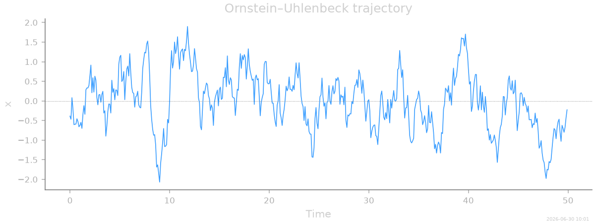
The trajectory shows the hallmark of a harmonic trap: the particle fluctuates around the origin, repeatedly pulled back by the restoring force.

Set up inference and estimate the diffusion

Inference runs through an engine built from the data — here OverdampedLangevinInference. The first quantity to pin down is the diffusion constant, which sets the noise scale and weights the force regression.

Our data is clean and free of measurement noise, so we use the plain mean-squared-displacement estimator, method="MSD", which is exact in the fine-sampling limit. On real recordings with localization noise, drop the argument: the default method="auto" then selects a noise-robust estimator instead (see Measurement noise and coarse sampling).

Note

More broadly, this tutorial uses SFI’s linear estimators throughout — the right choice for clean, finely-sampled data. For measurement noise, coarse sampling, or models nonlinear in their parameters, switch to the parametric estimators (infer_force() / infer_diffusion()); the regime table in Choosing an estimator tells you when.

inf = SFI.OverdampedLangevinInference(coll)
inf.compute_diffusion_constant(method="MSD")

Infer the force

Now the central step. In a real experiment we would not know that the force is linear, so we hand SFI a generic, deliberately over-complete library of candidate terms — the monomials \(\{1,\,x,\,x^2\}\) — and let the data decide which it needs. monomials_up_to() builds that basis; rank='vector' makes each term a force component.

from SFI.bases import monomials_up_to

B = monomials_up_to(order=2, dim=1, rank="vector")   # candidates: 1, x, x²

inf.infer_force_linear(B)        # closed-form regression onto the basis
inf.compute_force_error()        # predicted (sampling-noise) NMSE
inf.print_report()

  --- StochasticForceInference Report ---
Average diffusion tensor:
 [[0.5044536]]
Measurement noise tensor:
 [[0.0043071]]
Force estimated information: 11.061005592346191
Force: estimated normalized mean squared error (sampling only): 0.13561157212196093

  Force Coefficient Table
  ────────────────────────────────────────────────────────────────
  #    Label     Coefficient       Std.Err     SNR  Sig
  ────────────────────────────────────────────────────────────────
  0    1·e0      4.52164e-02   1.83873e-01     0.2  ·
  1    x0·e0    -9.68892e-01   2.06032e-01     4.7  *
  2    x0^2·e0  -7.57193e-02   2.19615e-01     0.3  ·
  ────────────────────────────────────────────────────────────────
  3/3 basis functions in support, sig: 1* / 0** / 0*** (|SNR| ≥ 2 / 10 / 100)
  (Std.err. reflects sampling error only; discretization bias is not included.)

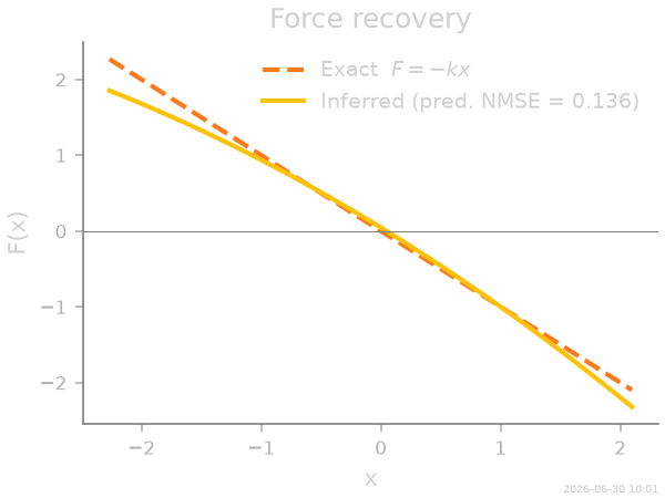
The report lists the fitted coefficients and a predicted normalized mean-squared error — SFI’s own estimate of how well the force is pinned down by this much data, available without any ground truth.

Because this is a synthetic benchmark we can check against the truth. The inferred force \(\hat F(x)\), with its 1-σ confidence band, overlays the exact \(F(x) = -k\,x\) almost perfectly.

x_jnp = jnp.array(np.linspace(Xarr.min() - 0.3, Xarr.max() + 0.3, 200)[:, None])

# capture the full-basis coefficients before model selection prunes them
coeffs_full = np.asarray(inf.force_coefficients_full)
stderr_full = np.asarray(inf.force_coefficients_stderr)

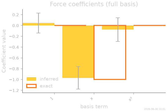
Which terms does the data support? Model selection

Our basis had three candidate terms, but only one — the linear term — is really present. Looking at the fitted coefficients with their 1-σ error bars already tells the story: the constant and quadratic terms are statistically indistinguishable from zero, while the linear coefficient sits squarely at \(-k\).

labels = ["1", "x", "x²"]
coeffs_exact = np.array([0.0, -k_true, 0.0])

Rather than read the bars by eye, let SFI make the choice. sparsify_force() runs a model search scored by an information criterion — the default is PASTIS, SFI’s parsimonious criterion — and keeps only the terms the data actually warrant.

inf.sparsify_force(criterion="PASTIS")
inf.compute_force_error()
inf.print_report()

  --- StochasticForceInference Report ---
Average diffusion tensor:
 [[0.5044536]]
Measurement noise tensor:
 [[0.0043071]]
Force estimated information: 11.001898765563965
Force: estimated normalized mean squared error (sampling only): 0.045446697961144825

  Force Coefficient Table
  ────────────────────────────────────────────────────────────────
  #    Label     Coefficient       Std.Err     SNR  Sig
  ────────────────────────────────────────────────────────────────
  1    x0·e0    -9.62484e-01   2.05185e-01     4.7  *
  ────────────────────────────────────────────────────────────────
  1/3 basis functions in support, sig: 1* / 0** / 0*** (|SNR| ≥ 2 / 10 / 100)
  (Std.err. reflects sampling error only; discretization bias is not included.)
  Zeroed (2): 1·e0, x0^2·e0

PASTIS keeps the single linear term and discards the constant and quadratic — recovering the exact structure of the model, not just its values. Selecting the minimal model both sharpens the estimate and makes it interpretable: the answer is “a harmonic trap”, stated in one coefficient.

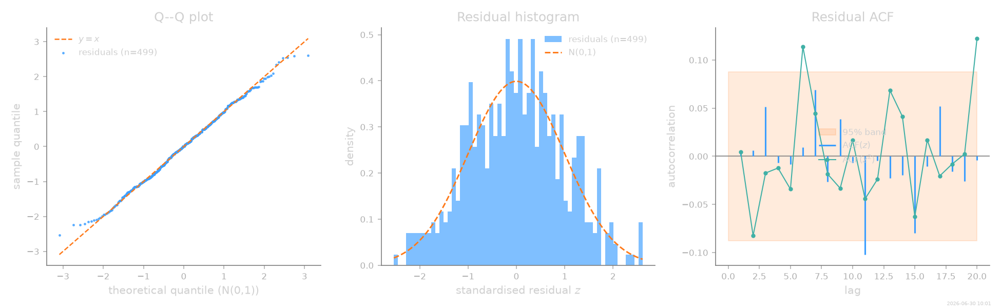
Consistency diagnostics

With real data there is no exact model to compare against, so the canonical sanity check is statistical. SFI recomputes the standardised residuals \(z_t = (\Delta x_t - \hat F(x_t)\,\Delta t)/\sqrt{2\hat D\,\Delta t}\) and asks whether they look like independent \(\mathcal N(0,1)\) draws. SFI.diagnostics.assess() (also reachable as inf.diagnose()) runs a panel of tests and returns a report.

from SFI.diagnostics import assess, plot_summary

report = assess(inf, level="standard")
report.print_summary()

=== SFI diagnostics report ===
backend  : linear
regime   : OD
n_obs    : 499  n_particles: 1  d: 1
level    : standard

-- Residuals --
  mean = +0.0015  std = 0.9768  skew = +0.037  kurt-3 = -0.329  (n=499)
  ✓ normality ks                 stat=0.0208    p=0.979
  ✓ autocorr  ljung_box          stat=16.1      p=0.711
  ✓ autocorr  ljung_box_squared  stat=27.5      p=0.121
  predicted NMSE = 0.0454  realised NMSE = 0  χ² z = -0.75 (|z|>5 ⇒ bias)

-- Flags --
  (no issues at α = 0.01)

A well-specified fit shows a pooled residual mean ≈ 0, standard deviation ≈ 1, no autocorrelation, normal tails, and a realised error consistent with the predicted one. Residual autocorrelation would point to missing dynamics; a standard deviation far from 1 to a mis-estimated diffusion. See the Diagnostics user guide for the full inventory.

Bootstrapped trajectory

A second, dynamical check: simulate a new trajectory directly from the inferred model. If the fit is faithful, this bootstrap should be statistically indistinguishable from the original data — same spread, same relaxation. Inferred models are first-class simulators, so this is a single call.

key_boot = random.PRNGKey(0)
coll_boot, _ = inf.simulate_bootstrapped_trajectory(key_boot)

_, Xb_full, _ = coll_boot.to_arrays(dataset=0)
Xb = Xb_full[:, 0, 0]                                 # bootstrapped x(t)

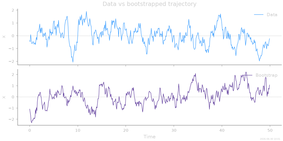
The trajectories look alike, but the sharper test is in statistics the fit never used directly. SFI only sees short-time increments \(\Delta x\) over one step dt; everything at longer lags — how fast correlations decay, how far the particle wanders — is a genuine prediction of the inferred model. Comparing those long-time statistics between the data and a bootstrap is one of the most informative consistency checks available without ground truth.

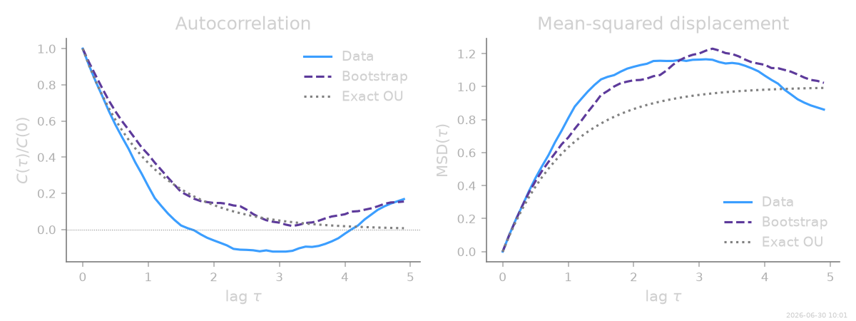
We look at two: the autocorrelation \(C(\tau) = \langle x(t)\,x(t+\tau)\rangle\) (how memory fades) and the mean-squared displacement \(\mathrm{MSD}(\tau) = \langle [x(t+\tau)-x(t)]^2\rangle\) (how far it spreads). For an OU process both are exact exponentials, drawn here as dotted references.

def acf(x, n_lags):
    x = x - x.mean()
    c = np.correlate(x, x, mode="full")[len(x) - 1:]
    return c[:n_lags] / c[0]

def msd(x, n_lags):
    return np.array([np.mean((x[k:] - x[:-k]) ** 2) if k else 0.0
                     for k in range(n_lags)])

n_lags = 50
lags = np.arange(n_lags) * dt
acf_data, acf_boot = acf(Xarr[:, 0], n_lags), acf(Xb, n_lags)
msd_data, msd_boot = msd(Xarr[:, 0], n_lags), msd(Xb, n_lags)
acf_exact = np.exp(-k_true * lags)                       # OU: C(τ)/C(0) = e^{-kτ}
msd_exact = 2 * (D_true / k_true) * (1 - np.exp(-k_true * lags))

#
# Data and bootstrap track each other and the exact OU curves across all
# lags: the inferred short-time force and diffusion reproduce the
# emergent long-time behaviour the fit never saw directly.

examples/gallery/ou_demo.py:346: UserWarning: The figure layout has changed to tight
  plt.tight_layout()

Save and load

Finally, persist the result. SFI offers two complementary serializers:

• save_results() writes a lightweight summary (coefficients, errors, metadata) as .npz + .json;

• save_model() writes the fitted callable model so the inferred force can be re-evaluated later. Reloading it needs a template that supplies the basis structure (the dictionary of functions is not pickled).

We write to a temporary directory here to keep the example self-contained.

import os
import tempfile

from SFI.inference import load_model, load_results, save_model, save_results

tmp = tempfile.mkdtemp()

# 1. lightweight summary
save_results(inf, os.path.join(tmp, "ou_inference"))
summary = load_results(os.path.join(tmp, "ou_inference"))
print("Reloaded summary keys:", sorted(summary)[:5], "...")

# 2. the callable force model
save_model(inf.force_inferred, os.path.join(tmp, "ou_force"))
force_reloaded = load_model(os.path.join(tmp, "ou_force"),
                            template=inf.force_inferred)

# the reloaded model evaluates to the same force
max_diff = float(np.max(np.abs(
    np.asarray(force_reloaded(x_jnp)) - np.asarray(inf.force_inferred(x_jnp))
)))
print(f"Reloaded model matches original (max |Δ| = {max_diff:.2e})")

Reloaded summary keys: ['Lambda', '_sfi_version', 'diffusion_average', 'force_coefficients', 'force_coefficients_full'] ...
Reloaded model matches original (max |Δ| = 0.00e+00)

Next steps

That is the full arc — simulate, infer, select, validate, persist — in a few dozen lines. Where to go next:

• Real experimental data follows the identical workflow; you skip the “exact model” comparison and lean on diagnostics and bootstrapping for validation. Start from Start here: is SFI right for my data? for the routing guide, then use Experimental-data workflow template as the template.

• Noisy or coarsely-sampled recordings need the parametric estimators — see Measurement noise and coarse sampling.

• Building models (custom bases, interactions, masking): Models and state functions and Building bases.

• Trajectory I/O (loading CSV/Parquet/HDF5, multi-experiment data): Trajectory data.

• Inference in depth (overdamped vs. underdamped, diffusion methods, error analysis): Running inference.

stamp_output()

[Generated: 2026-06-30 10:01]

🏷 Tags: synthetic, overdamped, linear, 1D