Note
Go to the end to download the full example code.
Learning a time-dependent force field — time-Fourier basis
Recover an unknown, time-varying force law from trajectories alone, by expanding time in a Fourier dictionary.
The companion Time-dependent forcing — protocols as extras infers a known, recorded drive. Here the drive is not recorded: a population of overdamped particles sits in a common harmonic trap whose centre \(a(t)\) and stiffness \(k(t)\) both wander in time,
SFI never sees \(k(t)\) or \(a(t)\). It is handed only the
trajectories and a time_fourier() dictionary, which
reads the auto-injected time clock (no protocol has to be
recorded). The linear estimator reconstructs both time-dependent
fields, and PASTIS keeps only the harmonics the data support.
Tags
synthetic · overdamped · linear · 1D · time-dependent
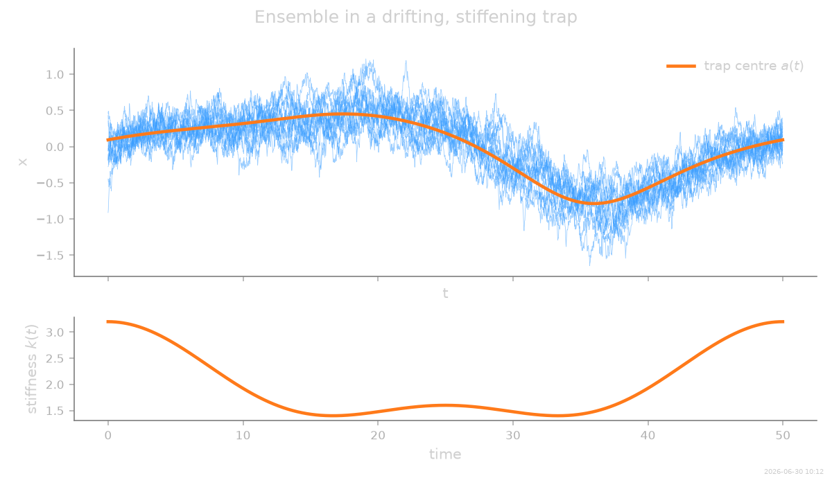
A trap that drifts and stiffens
The centre \(a(t)\) and stiffness \(k(t)\) are smooth but not single sinusoids — each is a short sum of harmonics of the fundamental \(\omega = 2\pi / T_\text{tot}\) (one period over the whole run). They are the ground truth we will try to recover; the estimator is never told them.
import SFI
from SFI.bases import X, time_fourier, unit_vector_basis, extra_scalar
from SFI.langevin import OverdampedProcess
from SFI.trajectory import time_series_extra
from SFI.utils.plotting import plot_time_profile_comparison, timeseries

dt = 0.02
Nframes = 2500
Nparticles = 48
D_true = 0.08

t = np.arange(Nframes) * dt
T_tot = t[-1]
w = 2 * np.pi / T_tot

k_t = 2.0 + 0.8 * np.cos(w * t) + 0.4 * np.cos(2 * w * t)   # stiffness > 0
b_t = 0.9 * np.sin(w * t) + 0.3 * np.cos(2 * w * t)         # additive drift k·a
a_t = b_t / k_t                                            # implied trap centre
Simulate an ensemble
A single trapped particle cannot separate “the trap is stiffer” from
“the trap has moved” — at any instant it just sits near the minimum.
A population breaks that degeneracy: at each time the spread of
particles around \(a(t)\) fixes the slope \(-k(t)\) and the
offset \(k(t)\,a(t)\). The particles are independent, so we
simulate Nparticles single-particle runs and merge them into one
ensemble collection.
F_true = extra_scalar("neg_k") * X(dim=1) & extra_scalar("drift") * unit_vector_basis(1)
proc = OverdampedProcess(F=F_true, D=D_true, theta_F=jnp.array([1.0, 1.0]))
proc.set_extras(extras_global={
    "neg_k": time_series_extra(-k_t),
    "drift": time_series_extra(b_t),
})

rng = np.random.default_rng(0)
runs = []
for i in range(Nparticles):
    proc.initialize(jnp.array([float(rng.normal() * 0.4)]))
    ci = proc.simulate(dt=dt, Nsteps=Nframes, key=random.PRNGKey(i),
                       oversampling=3, compute_observables=False)
    runs.append(ci)

coll = runs[0].merge(runs[1:])   # ensemble = many single-particle datasets
print(f"ensemble: {coll.datasets[0].T} frames x {Nparticles} particles")
ensemble: 2500 frames x 48 particles
Inference with a time-Fourier dictionary
Tensor a Fourier-in-time dictionary with the spatial terms:
time_fourier(n) * X carries the stiffness, and
time_fourier(n) * unit_vector_basis(1) the moving centre.
time_fourier() reads the auto-injected time extra;
with period=None its fundamental is the full trajectory duration.
Nothing about \(a(t)\) or \(k(t)\) is supplied.
n_modes = 6
B = time_fourier(n_modes) * X(dim=1) & time_fourier(n_modes) * unit_vector_basis(1)

inf = SFI.OverdampedLangevinInference(coll)
inf.compute_diffusion_constant(method="MSD")
inf.infer_force_linear(B)
inf.compute_force_error()
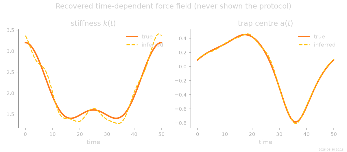
Reconstructed stiffness and centre
The two coefficient blocks give the time functions \(-k(t)\) (the
x block) and \(k(t)\,a(t)\) (the constant block); dividing
recovers the centre. Both match the hidden ground truth.
examples/gallery/time_fourier_demo.py:196: UserWarning: The figure layout has changed to tight
  fig.tight_layout()
k(t) reconstruction NMSE = 0.0024
a(t) reconstruction NMSE = 0.0012
Sparse selection of harmonics
The dictionary offers n_modes harmonics per spatial term, but the
data support only a few. PASTIS prunes the rest — the surviving
terms are exactly the harmonics built into \(k(t)\) and
\(k(t)\,a(t)\).
inf.sparsify_force(criterion="PASTIS")
inf.print_report()
  --- StochasticForceInference Report ---
Average diffusion tensor:
 [[0.0788167]]
Measurement noise tensor:
 [[6.256998e-05]]
Force estimated information: 1186.5589599609375
Force: estimated normalized mean squared error (sampling only): 0.010956048988142434

  Force Coefficient Table
  ────────────────────────────────────────────────────────────────────
  #    Label         Coefficient       Std.Err     SNR  Sig
  ────────────────────────────────────────────────────────────────────
  0    1·x          -1.97601e+00   4.13784e-02    47.8  **
  1    cos(1wt)·x   -8.41564e-01   6.12111e-02    13.7  **
  3    cos(2wt)·x   -4.20467e-01   5.81531e-02     7.2  *
  15   sin(1wt)·e0   8.69886e-01   2.77417e-02    31.4  **
  16   cos(2wt)·e0   3.03681e-01   2.46001e-02    12.3  **
  ────────────────────────────────────────────────────────────────────
  5/26 basis functions in support, sig: 5* / 4** / 0*** (|SNR| ≥ 2 / 10 / 100)
  (Std.err. reflects sampling error only; discretization bias is not included.)
  Zeroed (21): sin(1wt)·x, sin(2wt)·x, cos(3wt)·x, sin(3wt)·x, cos(4wt)·x, sin(4wt)·x, cos(5wt)·x, sin(5wt)·x, cos(6wt)·x, sin(6wt)·x, 1·e0, cos(1wt)·e0, sin(2wt)·e0, cos(3wt)·e0, sin(3wt)·e0, cos(4wt)·e0, sin(4wt)·e0, cos(5wt)·e0, sin(5wt)·e0, cos(6wt)·e0, sin(6wt)·e0
Notes
Time as an extra. The reserved
timeextra is injected automatically, per frame, by the trajectory layer (seebuild_extras()), sotime_fourier()needs no recorded protocol. Withperiod=Nonethe fundamental is the full trajectory duration; passperiod=to fit a known repeat time.Why an ensemble. The stiffness and the centre are jointly identifiable only because many particles sample a spread of positions at each instant; a single tightly-trapped trajectory cannot tell a stiffer trap from a displaced one.
Beyond traps. Any time-dependent force field — ramps, oscillatory drives, slow aging — can be learned the same way: tensor
time_fourier()with whatever spatial basis the problem needs, and let PASTIS keep the active modes.
stamp_output()
[Generated: 2026-06-30 10:13]
Total running time of the script: (0 minutes 31.602 seconds)