Experimental-data workflow template

The recommended workflow for applying SFI to real experimental data. This demo loads a 2D optical-tweezer trajectory from a CSV file, infers the force and diffusion, sparsifies with PASTIS, and validates with a bootstrap trajectory.

The data includes localization noise, a slow rotation (torque), and a weak Duffing-type cubic anharmonicity in \(x\). PASTIS automatically detects these non-trivial terms beyond the harmonic restoring force.

SFI’s design philosophy

Stochastic Force Inference is built for experimental trajectories where no model pre-exists. The linear regression backbone requires no initial guess, works with arbitrary basis functions, and the PASTIS information criterion rigorously identifies which terms are supported by the data.

Tags

real-data · overdamped · experimental-workflow

Step 1 — Load trajectory from CSV

TrajectoryCollection.load() handles CSV (with optional YAML header), Parquet, and HDF5. The CSV file here uses a # dt: 0.01 YAML header so the timestep is automatically set.

In your own workflow, replace the path with your data file.

from SFI.trajectory import TrajectoryCollection

csv_path = _here.parent / "experimental_data" / "optical_tweezer.csv"
coll = TrajectoryCollection.load(csv_path)

print(f"Loaded: {coll.T} frames, d={coll.d}, dt={coll.dt}")

Loaded: 20001 frames, d=2, dt=0.01

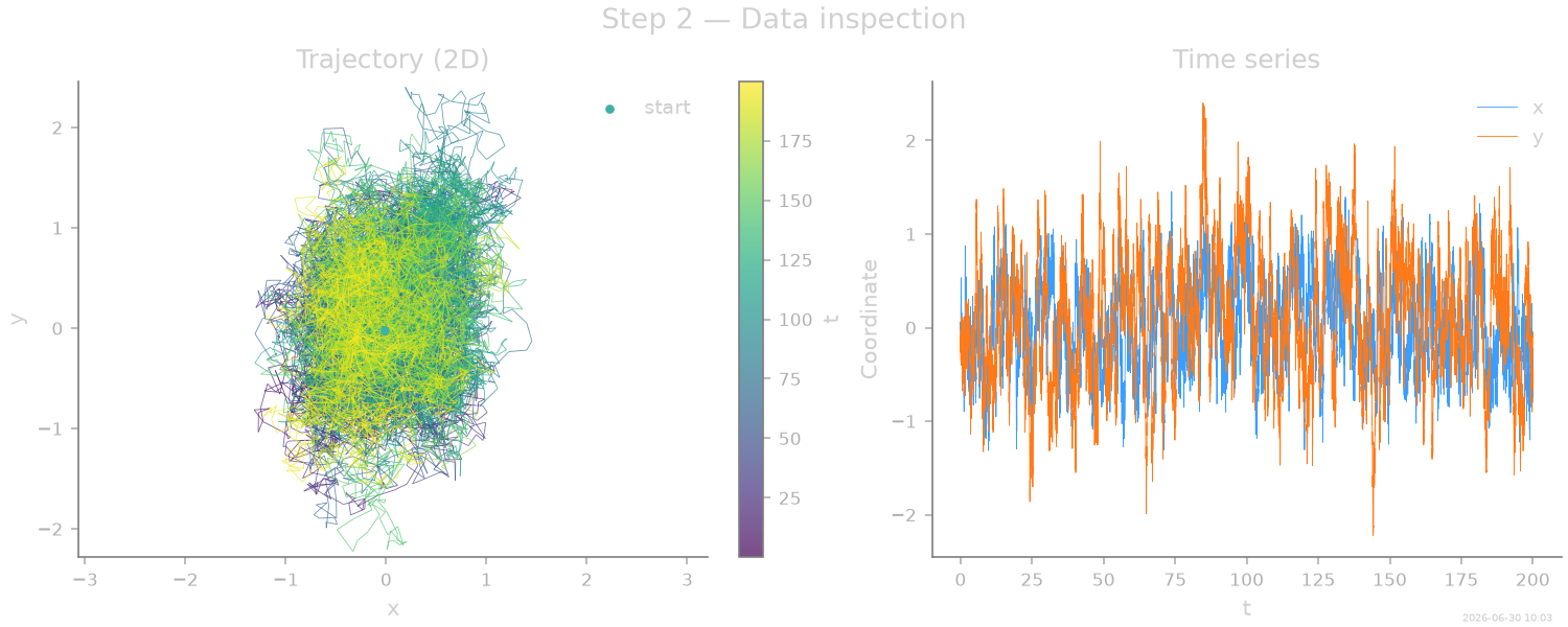
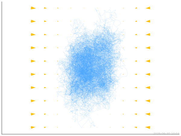
Step 2 — Visualize the data

Always inspect your data first: check for outliers, missing frames, or obvious drift.

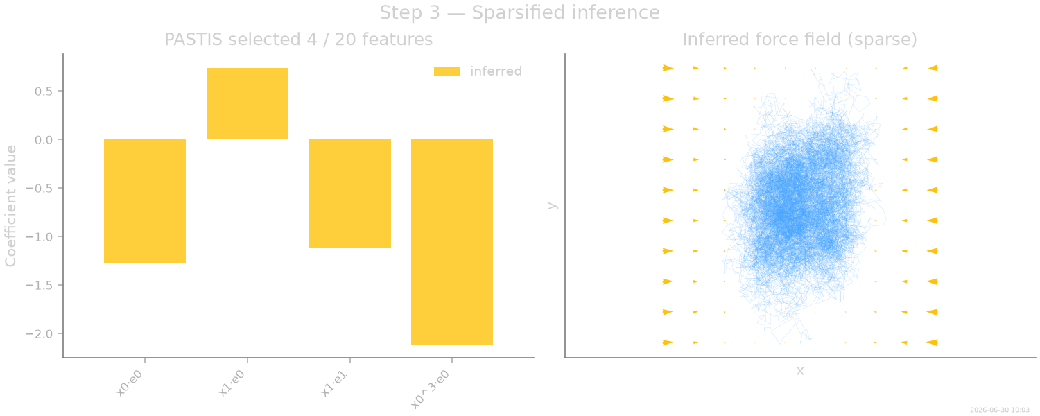
Step 3 — Basis, inference, and sparsification

Start with a polynomial basis (degree 3). For experimental data you typically do not know the diffusion tensor, so we estimate it. PASTIS then selects the simplest model the data supports.

The data contains a weak Duffing cubic (\(-\alpha\,x^3\)) in one axis and a slow rotation; PASTIS should recover these beyond the dominant harmonic terms.

from SFI.bases import monomials_up_to
from SFI import OverdampedLangevinInference
from SFI.utils import plotting

degree = 3
B = monomials_up_to(order=degree, dim=2, rank='vector')

inf = OverdampedLangevinInference(coll)
inf.compute_diffusion_constant()
inf.infer_force_linear(B)
inf.compute_force_error()

inf.sparsify_force(criterion="PASTIS")
support = np.asarray(inf.force_support)
k_sel = len(support)
if k_sel > 0:
    inf.compute_force_error()

inf.print_report()

  --- StochasticForceInference Report ---
Average diffusion tensor:
 [[0.48866063 0.00630378]
 [0.00630378 0.5060318 ]]
Measurement noise tensor:
 [[ 5.5156957e-04 -6.7758949e-05]
 [-6.7758949e-05  5.2479864e-04]]
Force estimated information: 197.58346557617188
Force: estimated normalized mean squared error (sampling only): 0.010122304486196823

  Force Coefficient Table
  ─────────────────────────────────────────────────────────────────────
  #    Label          Coefficient       Std.Err     SNR  Sig
  ─────────────────────────────────────────────────────────────────────
  2    x0·e0         -1.27470e+00   2.77786e-01     4.6  *
  4    x1·e0          7.40408e-01   1.05972e-01     7.0  *
  5    x1·e1         -1.11140e+00   1.05428e-01    10.5  **
  12   x0^3·e0       -2.10942e+00   4.44976e-01     4.7  *
  ─────────────────────────────────────────────────────────────────────
  4/20 basis functions in support, sig: 4* / 1** / 0*** (|SNR| ≥ 2 / 10 / 100)
  (Std.err. reflects sampling error only; discretization bias is not included.)
  Zeroed (16): 1·e0, 1·e1, x0·e1, x0^2·e0, x0^2·e1, (x0·x1)·e0, (x0·x1)·e1, x1^2·e0, x1^2·e1, x0^3·e1, (x0^2·x1)·e0, (x0^2·x1)·e1, (x0·x1^2)·e0, (x0·x1^2)·e1, x1^3·e0, x1^3·e1

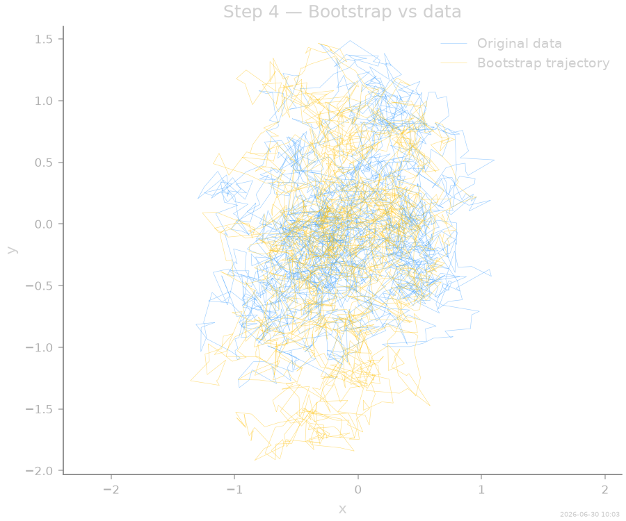
Step 4 — Bootstrap validation

Simulate a trajectory from the inferred model and compare with the original data — a self-consistency check.

key = random.PRNGKey(123)
coll_boot, _ = inf.simulate_bootstrapped_trajectory(key)

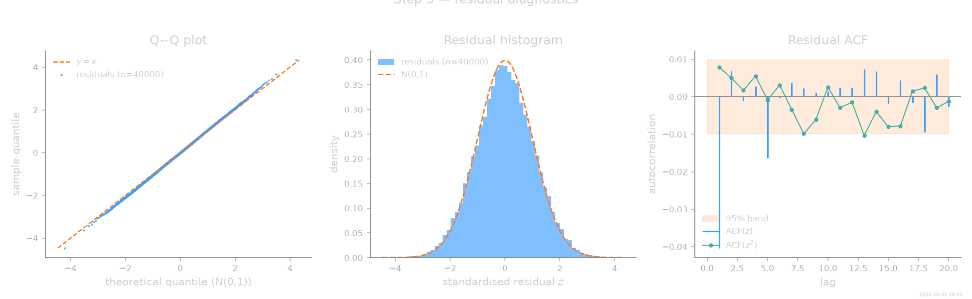
Step 5 — Consistency diagnostics

The final check on real data: recompute the standardised residuals and test whether they behave like an i.i.d. \(\mathcal{N}(0, 1)\) sample. Localization noise biases the linear Itô estimator (an errors-in-variables effect), so a residual-consistency flag here is a useful signal — not a failure of the workflow, but a sign that measurement noise matters for this dataset. When it appears, the parametric estimator (infer_force()) profiles the noise level and removes the bias — see Measurement noise and coarse sampling. Each flag below carries its one-line action hint inline.

from SFI.diagnostics import assess, plot_summary

report = assess(inf, level="standard")
report.print_summary()

=== SFI diagnostics report ===
backend  : linear
regime   : OD
n_obs    : 20000  n_particles: 1  d: 2
level    : standard

-- Residuals --
  mean = +0.0039  std = 1.0469  skew = +0.003  kurt-3 = -0.027  (n=40000)
  ✗ normality ks                 stat=0.014     p=3.29e-07
  ✗ autocorr  ljung_box          stat=90        p=7.48e-11
  ✓ autocorr  ljung_box_squared  stat=22.4      p=0.318
  predicted NMSE = 0.0101  realised NMSE = 9.41  χ² z = +13.58 (|z|>5 ⇒ bias)

-- Flags --
  ! [normality/ks] p=3.29e-07 < 0.01 — non-Gaussian residuals — rare events not captured by the basis, or a non-Gaussian noise structure
  ! [autocorr/ljung_box] p=7.48e-11 < 0.01 — missing time-correlated feature — widen the basis; if it persists, suspect coarse sampling: the parametric estimator (infer_force) extends the usable Δt
  ! [mse_consistency] residual chi^2 z-score = +13.58, realised/predicted NMSE = 9.3e+02 — realised error above predicted — model bias; on experimental data usually measurement noise: consider the parametric estimator (infer_force)

Thumbnail

stamp_output()

[Generated: 2026-06-30 10:03]

🏷 Tags: real-data, overdamped, experimental-workflow