Lorenz attractor — overdamped inference¶

Infer the force field of a 3D Lorenz system from a single simulated trajectory using polynomial basis functions.

This example demonstrates the full SFI workflow on a classic chaotic system: simulate → infer → sparsify → validate → bootstrap.

System definition¶

The classic chaotic Lorenz system:

\[\dot{x} = \sigma(y - x), \quad \dot{y} = x(\rho - z) - y, \quad \dot{z} = x\,y - \beta\,z\]

with \((\sigma, \rho, \beta) = (20, 8, 2)\), i.e. closer to the critical point than the classic parameters. We add isotropic noise \(D_0 = 5\) and simulate a short trajectory.

from SFI.bases import named_scalars, unit_axes, x_components
from SFI.langevin import OverdampedProcess
from SFI.utils import plotting

# Ground-truth Lorenz force, written directly as a symbolic composition
# of the basis primitives (no ``make_sf``, no raw array math).  Named
# scalars carry the reference parameter values as defaults, so the
# simulator can bind them automatically.
x, y, z = x_components(3)
ex, ey, ez = unit_axes(3)
sigma_p, rho_p, beta_p = named_scalars(sigma=20.0, rho=8.0, beta=2.0)

F_true = (
    (sigma_p * (y - x)) * ex
    + (x * (rho_p - z) - y) * ey
    + (x * y - beta_p * z) * ez
)

D0 = 5.0
dt = 0.005
Nsteps = 2000
seed = 0

key = random.PRNGKey(seed)

proc = OverdampedProcess(F_true, D=jnp.eye(3) * D0)
proc.initialize(jnp.array([1.0, 1.0, 1.0], dtype=jnp.float32))

key, sub = random.split(key)
coll = proc.simulate(dt=dt, Nsteps=Nsteps, key=sub, prerun=2000, oversampling=10)

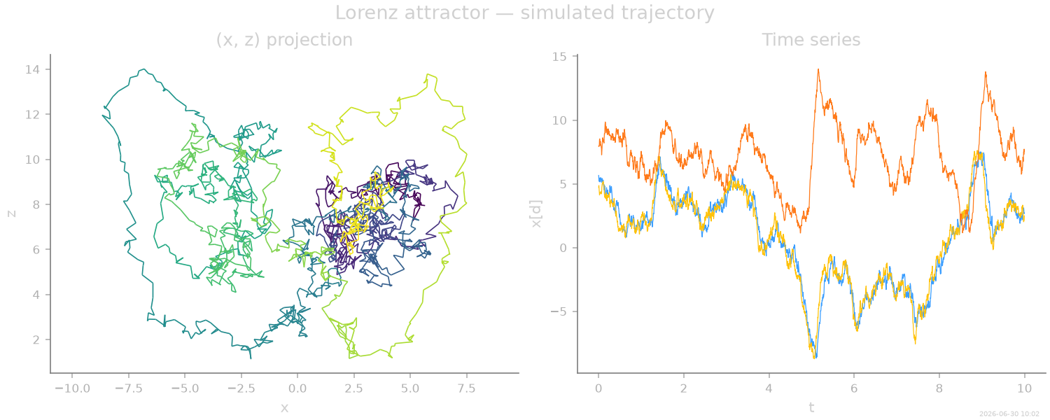
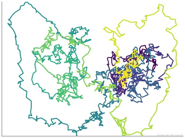
Trajectory¶

The characteristic butterfly structure is visible even on a short, noisy trajectory.

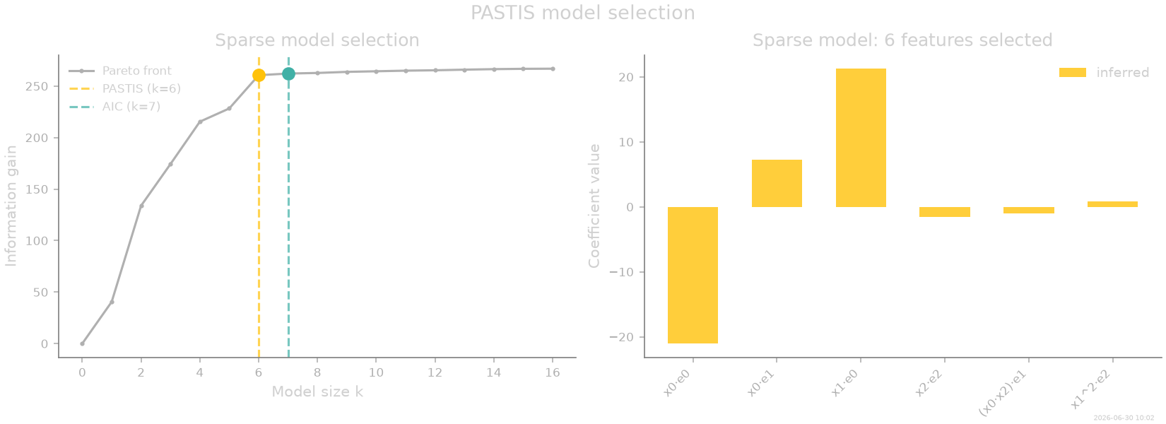
Inference and sparsification¶

A degree-2 polynomial basis in 3D gives 30 features. PASTIS sparsification recovers the 7-term Lorenz model.

from SFI.bases import monomials_up_to
from SFI import OverdampedLangevinInference

degree = 2
B = monomials_up_to(order=degree, dim=3, rank='vector')

inf = OverdampedLangevinInference(coll)
inf.compute_diffusion_constant(method="auto")
inf.infer_force_linear(B, M_mode="Ito", G_mode="trapeze")
inf.compute_force_error()

inf.sparsify_force(criterion="PASTIS")
inf.compute_force_error()
inf.compare_to_exact(model_exact=proc, maxpoints=2000)

inf.print_report()

  --- StochasticForceInference Report ---
Average diffusion tensor:
 [[ 4.915028   -0.09412182  0.08179999]
 [-0.09412178  4.9277186   0.17238185]
 [ 0.08179997  0.17238186  4.798985  ]]
Measurement noise tensor:
 [[-0.00089405 -0.00341186  0.00121787]
 [-0.00341186 -0.00330502  0.00119478]
 [ 0.00121787  0.00119478 -0.00447237]]
Force estimated information: 260.56060791015625
Force: estimated normalized mean squared error (sampling only): 0.01151363418754868
Normalized MSE (force):     0.0250
Normalized MSE (diffusion): 0.0022

  Force Coefficient Table
  ───────────────────────────────────────────────────────────────────
  #    Label        Coefficient       Std.Err     SNR  Sig
  ───────────────────────────────────────────────────────────────────
  3    x0·e0       -2.10495e+01   1.30301e+00    16.2  **
  4    x0·e1        7.26645e+00   9.01159e-01     8.1  *
  6    x1·e0        2.12654e+01   1.31485e+00    16.2  **
  11   x2·e2       -1.55772e+00   1.72741e-01     9.0  *
  19   (x0·x2)·e1  -9.90525e-01   1.07576e-01     9.2  *
  23   x1^2·e2      8.89709e-01   6.97303e-02    12.8  **
  ───────────────────────────────────────────────────────────────────
  6/30 basis functions in support, sig: 6* / 3** / 0*** (|SNR| ≥ 2 / 10 / 100)
  (Std.err. reflects sampling error only; discretization bias is not included.)
  Zeroed (24): 1·e0, 1·e1, 1·e2, x0·e2, x1·e1, x1·e2, x2·e0, x2·e1, x0^2·e0, x0^2·e1, x0^2·e2, (x0·x1)·e0, (x0·x1)·e1, (x0·x1)·e2, (x0·x2)·e0, (x0·x2)·e2, x1^2·e0, x1^2·e1, (x1·x2)·e0, (x1·x2)·e1, (x1·x2)·e2, x2^2·e0, x2^2·e1, x2^2·e2

Pareto front and sparse model¶

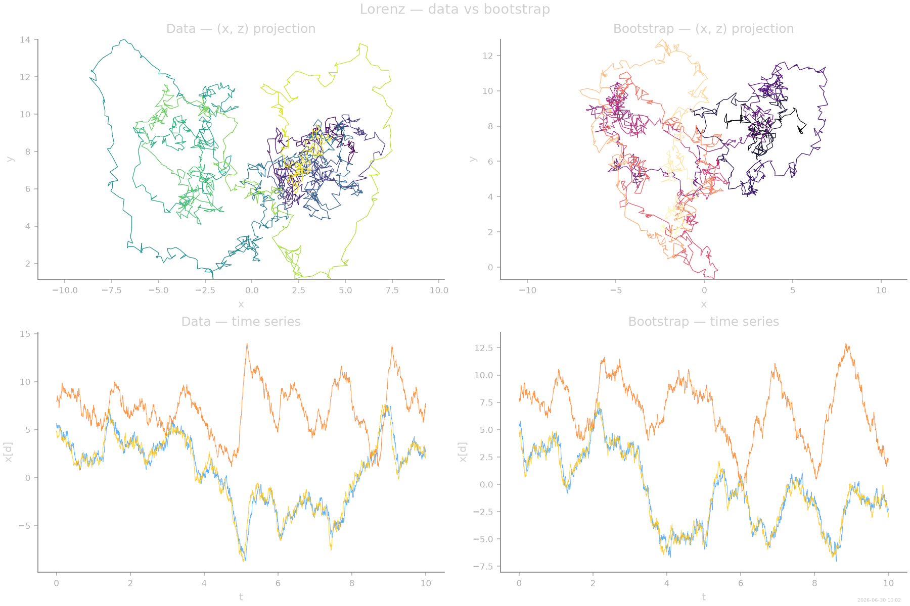
PASTIS model selection, Sparse model selection, Sparse model: 6 features selected

Bootstrap trajectory¶

Generate a bootstrapped trajectory from the inferred sparse model.

key_boot = random.PRNGKey(seed + 99)
coll_boot, _ = inf.simulate_bootstrapped_trajectory(key_boot, oversampling=10)

Data vs bootstrap comparison¶

Phase-space projection and time series of the data (top) vs the bootstrapped trajectory (bottom), straight from the toolkit plotters on each collection.

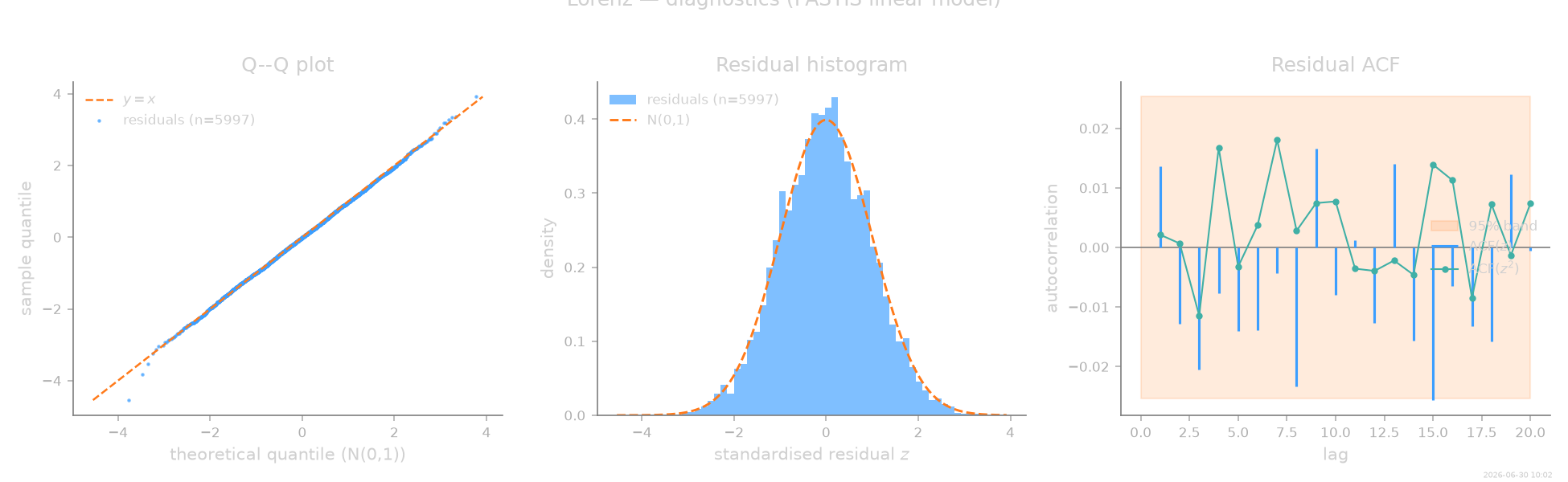
Lorenz — data vs bootstrap, Data — (x, z) projection, Bootstrap — (x, z) projection, Data — time series, Bootstrap — time series

Diagnostics¶

Once a fit is in hand, assess() recomputes standardised residuals \(z_t = (\Delta x_t - \hat F(x_t)\,\Delta t)/\sqrt{2\hat D\,\Delta t}\) and runs a panel of statistical tests. A well-specified model should have residuals that are i.i.d. \(\mathcal{N}(0,1)\) — no autocorrelation, no excess kurtosis, and a realised NMSE consistent with the predicted (sampling-noise) value.

Here we diagnose the PASTIS-selected linear model (Itô estimator).

from SFI.diagnostics import assess, plot_summary

report = assess(inf, level="standard")
report.print_summary()

Lorenz — diagnostics (PASTIS linear model), Q--Q plot, Residual histogram, Residual ACF

=== SFI diagnostics report ===
backend  : linear
regime   : OD
n_obs    : 1999  n_particles: 1  d: 3
level    : standard

-- Residuals --
  mean = -0.0120  std = 0.9882  skew = +0.001  kurt-3 = +0.098  (n=5997)
  ✓ normality ks                 stat=0.0131    p=0.25
  ✓ autocorr  ljung_box          stat=24.1      p=0.239
  ✓ autocorr  ljung_box_squared  stat=8.68      p=0.986
  predicted NMSE = 0.0115  realised NMSE = 0  χ² z = -1.29 (|z|>5 ⇒ bias)

-- Flags --
  (no issues at α = 0.01)

Thumbnail¶

stamp_output()

[Generated: 2026-06-30 10:02]

Total running time of the script: (0 minutes 23.772 seconds)

🏷 Tags: synthetic, overdamped, nonlinear, sparsity, 3D, benchmark

Gallery generated by Sphinx-Gallery