Van der Pol oscillator — underdamped inference¶

Infer the force field of a 1D Van der Pol oscillator from position-only data. Velocities are reconstructed internally by the ULI estimators.

This example demonstrates underdamped Langevin inference: the system has inertia, but only positions are observed — as is typical for experimental tracking data.

System definition¶

The Van der Pol oscillator:

\[\ddot{x} = \mu (1 - x^2)\,\dot{x} - x + \sqrt{2D}\,\xi(t)\]

with $\mu = 3$ (strongly nonlinear) and $D_0 = 0.05$. We use a time step $\Delta t = 5 \times 10^{-3}$ and a long trajectory to capture ~10 complete oscillation cycles.

from SFI.bases import named_scalar, unit_axes, v_components, x_components
from SFI.langevin import UnderdampedProcess
from SFI.utils import plotting

mu = 3.0
D0 = 0.05
dt = 0.02
Nsteps = 2000
oversampling = 8  # fine substeps → accurate Verlet integration of the SDE
seed_data = 0

# Ground-truth force written compositionally:
#     F(x, v) = mu * (1 - x²) * v - x
# Named scalar carries the reference value as a default, so the
# simulator binds the parameter automatically.
(_x,) = x_components(1)
(_v,) = v_components(1)
(_ex,) = unit_axes(1)
mu_p = named_scalar("mu", default=mu)
F_exact = (mu_p * (1 - _x * _x) * _v - _x) * _ex

key = random.PRNGKey(seed_data)
proc = UnderdampedProcess(F_exact, D=jnp.array([[D0]]))
proc.initialize(jnp.array([1.0]), v0=jnp.array([0.0]))

key, sub = random.split(key)
coll = proc.simulate(dt=dt, Nsteps=Nsteps, key=sub, prerun=200, oversampling=oversampling)

t, X, _ = coll.to_arrays(dataset=0)   # t:(T,), X:(T, N, d)
x = X[:, 0, 0]

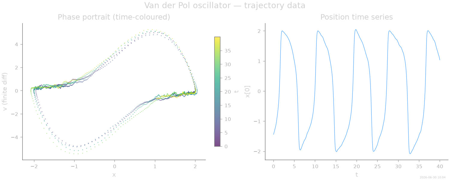
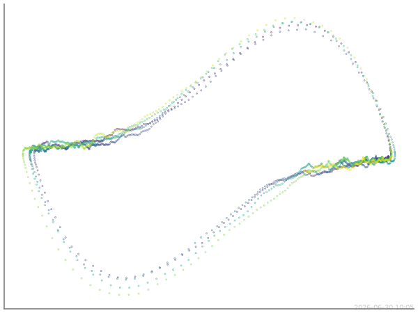
Phase portrait¶

The Van der Pol limit cycle in the $(x, \dot{x})$ plane. Velocities are estimated via finite differences for visualisation; the inference engine uses more sophisticated ULI reconstructions.

Force inference¶

Monomials in $(x, v)$ up to degree 3 capture the cubic nonlinearity. UnderdampedLangevinInference handles velocity reconstruction, diffusion estimation, and force projection.

from SFI.bases import monomials_up_to
from SFI import UnderdampedLangevinInference

degree = 3
B = monomials_up_to(order=degree, dim=1, include_v=True, rank='vector')

inf = UnderdampedLangevinInference(coll)
inf.compute_diffusion_constant()
# Default preset="auto": this trajectory is clean (Lambda_trace < 0), so the
# auto switch selects the sharper "clean"/WeakNoise estimator on its own.
inf.infer_force_linear(B)
inf.compute_force_error()
inf.compare_to_exact(model_exact=proc, data_exact=coll, maxpoints=2000)

inf.print_report()

  --- StochasticForceInference Report ---
Average diffusion tensor:
 [[0.05549547]]
Measurement noise tensor:
 [[-4.8412693e-07]]
Force estimated information: 4455.1044921875
Force: estimated normalized mean squared error (sampling only): 0.001122307275636466
Normalized MSE (force):     0.0229
Normalized MSE (diffusion): 0.0098

  Force Coefficient Table
  ─────────────────────────────────────────────────────────────────────
  #    Label          Coefficient       Std.Err     SNR  Sig
  ─────────────────────────────────────────────────────────────────────
  0    1·e0          -2.44047e-01   1.78127e-01     1.4  ·
  1    x0·e0         -9.87828e-01   1.56945e-01     6.3  *
  2    v0·e0          4.52392e+00   1.58589e-01    28.5  **
  3    x0^2·e0        1.18769e-01   5.85006e-02     2.0  *
  4    (x0·v0)·e0    -4.98457e-02   6.97995e-02     0.7  ·
  5    v0^2·e0        1.80063e-02   2.03494e-02     0.9  ·
  6    x0^3·e0       -1.16508e-01   4.68651e-02     2.5  *
  7    (x0^2·v0)·e0  -4.26904e+00   1.00399e-01    42.5  **
  8    (x0·v0^2)·e0   5.84279e-01   5.35458e-02    10.9  **
  9    v0^3·e0       -1.27913e-01   1.23059e-02    10.4  **
  ─────────────────────────────────────────────────────────────────────
  10/10 basis functions in support, sig: 7* / 4** / 0*** (|SNR| ≥ 2 / 10 / 100)
  (Std.err. reflects sampling error only; discretization bias is not included.)

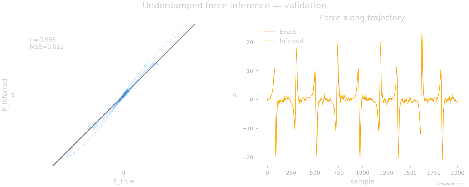
Force validation¶

Scatter plot of exact vs inferred force, evaluated along the ULI-reconstructed trajectory.

F_true, F_pred = inf.force_comparison_arrays(model_exact=proc)

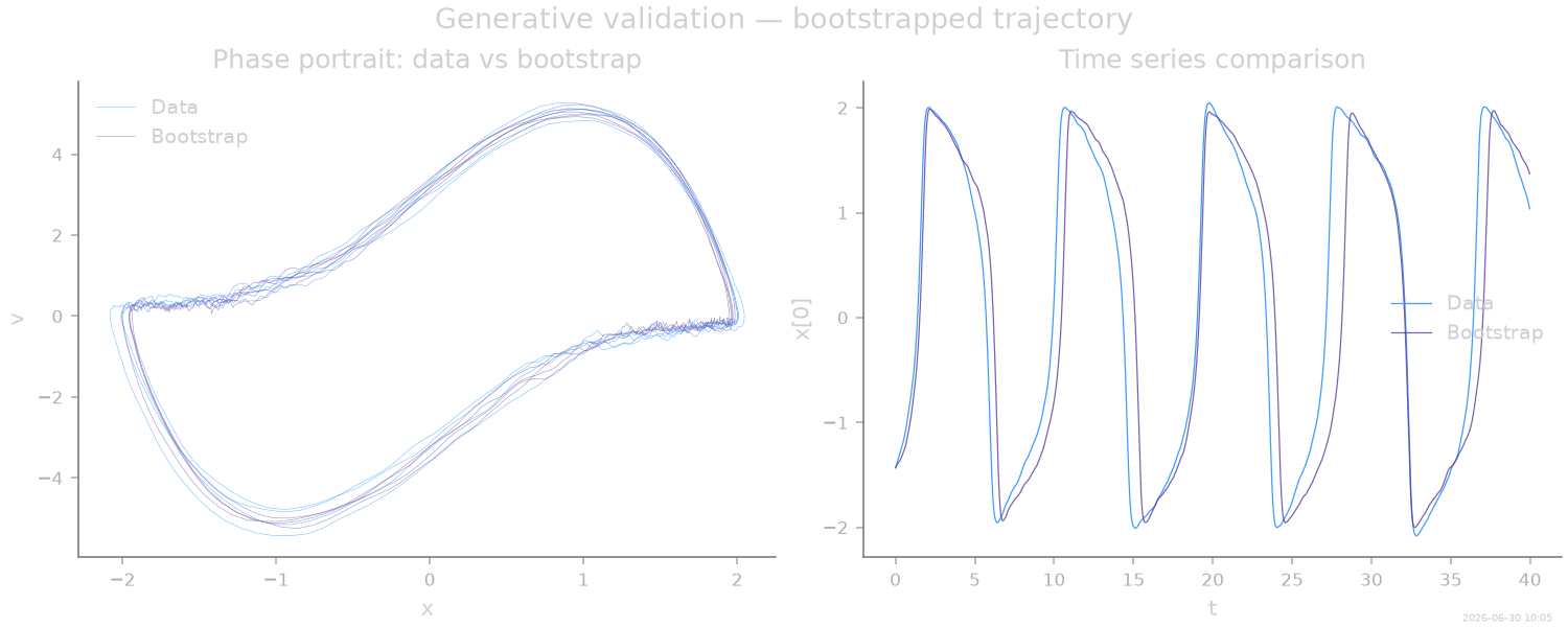
Underdamped force inference — validation, $r=0.993$ MSE=0.012, Force along trajectory

Bootstrapped trajectory¶

Simulating from the inferred model and comparing the phase portrait provides a generative validation.

key_boot = random.PRNGKey(1)
coll_boot, _ = inf.simulate_bootstrapped_trajectory(
    key_boot, oversampling=oversampling, simulate=True
)
_, X_boot, _ = coll_boot.to_arrays(dataset=0)
x_boot = X_boot[:, 0, 0]
v_fd_boot = coll_boot.velocity_array(dataset=0, scheme="central")[:, 0, 0]

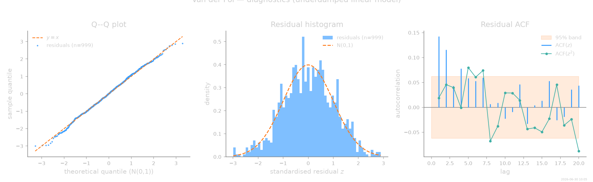
Generative validation — bootstrapped trajectory, Phase portrait: data vs bootstrap, Time series comparison

Diagnostics¶

The underdamped residual compares the symmetric finite-difference acceleration $\hat a = (x_{t+1} - 2x_t + x_{t-1})/\Delta t^2$ (the same kinematic the force estimator fits) to the inferred force $\hat F(\hat x, \hat v)$, standardised by the noise scale of a second difference of integrated white noise, $\tfrac23\,(2\hat D)/\Delta t$. Adjacent accelerations overlap, so every second sample is used to keep the residuals independent. A well-specified cubic-in-$(x,v)$ model then passes all checks.

from SFI.diagnostics import assess, plot_summary

report = assess(inf, level="standard")
report.print_summary()

Van der Pol — diagnostics (underdamped linear model), Q--Q plot, Residual histogram, Residual ACF

=== SFI diagnostics report ===
backend  : linear
regime   : UD
n_obs    : 999  n_particles: 1  d: 1
level    : standard

-- Residuals --
  mean = +0.0221  std = 1.0195  skew = -0.071  kurt-3 = -0.129  (n=999)
  ✓ normality ks                 stat=0.0294    p=0.347
  ✗ autocorr  ljung_box          stat=62.9      p=2.54e-06
  ✗ autocorr  ljung_box_squared  stat=46.1      p=0.00078
  predicted NMSE = 0.00112  realised NMSE = 0.00534  χ² z = +0.87 (|z|>5 ⇒ bias)

-- Flags --
  ! [autocorr/ljung_box] p=2.54e-06 < 0.01 — missing time-correlated feature — widen the basis; if it persists, suspect coarse sampling: the parametric estimator (infer_force) extends the usable Δt
  ! [autocorr/ljung_box_squared] p=7.80e-04 < 0.01 — diffusion mis-estimated or state-dependent — try the other compute_diffusion_constant method or a state-dependent diffusion basis; the parametric estimators profile (D, Λ)

Thumbnail¶

stamp_output()

[Generated: 2026-06-30 10:05]

Total running time of the script: (0 minutes 17.277 seconds)

🏷 Tags: synthetic, underdamped, nonlinear, 1D

Gallery generated by Sphinx-Gallery