Diagnostics — assessing fit quality

Once a fit is in hand, the next question is should we trust it? The SFI.diagnostics submodule answers that by recomputing standardised innovations from the fitted state function and the inferred constant diffusion, then running a battery of statistical tests.

This demo fits two models to the same 1-D double-well trajectory:

1. a well-specified cubic basis \(\{1, x, x^2, x^3\}\), and

2. a deliberately wrong linear basis \(\{1, x\}\) (missing the cubic term),

and contrasts their diagnostic reports side-by-side.

Tags

diagnostics · overdamped · linear · 1D · synthetic

Simulate a 1-D double-well process

A standard test bed for misspecification: \(F(x) = x - x^3\) has a cubic restoring force with two stable fixed points at \(x = \pm 1\). We sample at a moderate \(\Delta t = 0.05\) — coarse enough that a missing force term leaves a residual the diagnostics can detect (see the closing note on sampling interval).

import SFI
from SFI.bases import monomials_up_to, unit_axes, x_components
from SFI.diagnostics import assess, plot_summary
from SFI.langevin import OverdampedProcess

# Double-well force F(x) = x − x³, written compositionally.
(_x,) = x_components(1)
(_ex,) = unit_axes(1)
F_sf = (_x - _x * _x * _x) * _ex

proc = OverdampedProcess(F_sf, D=0.15)
proc.initialize(jnp.array([0.5], dtype=jnp.float32))
coll = proc.simulate(
    dt=0.05, Nsteps=8000, key=random.PRNGKey(2), prerun=200, oversampling=10,
)

Fit (1): well-specified cubic basis

inf_good = SFI.OverdampedLangevinInference(coll)
inf_good.compute_diffusion_constant(method="WeakNoise")
B_good = monomials_up_to(order=3, dim=1, rank='vector')  # {1, x, x², x³}
inf_good.infer_force_linear(B_good, M_mode="Ito")
inf_good.compute_force_error()

Fit (2): deliberately misspecified — linear force only (no cubic)

inf_bad = SFI.OverdampedLangevinInference(coll)
inf_bad.compute_diffusion_constant(method="WeakNoise")
B_bad = monomials_up_to(order=1, dim=1, rank='vector')  # {1, x} — misses x³
inf_bad.infer_force_linear(B_bad, M_mode="Ito")
inf_bad.compute_force_error()

Run diagnostics on both

Each flagged issue in the -- Flags -- block carries a one-line action hint pointing at the likely cure.

rep_good = assess(inf_good, level="standard")
rep_bad = assess(inf_bad, level="standard")

print("\n### Well-specified fit ###")
rep_good.print_summary()

print("\n### Misspecified fit ###")
rep_bad.print_summary()

### Well-specified fit ###

=== SFI diagnostics report ===
backend  : linear
regime   : OD
n_obs    : 7999  n_particles: 1  d: 1
level    : standard

-- Residuals --
  mean = +0.0000  std = 0.9617  skew = +0.007  kurt-3 = -0.018  (n=7999)
  ✓ normality ks                 stat=0.0115    p=0.243
  ✓ autocorr  ljung_box          stat=21.5      p=0.367
  ✓ autocorr  ljung_box_squared  stat=35.8      p=0.0164
  predicted NMSE = 0.0114  realised NMSE = 0  χ² z = -4.76 (|z|>5 ⇒ bias)

-- Flags --
  (no issues at α = 0.01)


### Misspecified fit ###

=== SFI diagnostics report ===
backend  : linear
regime   : OD
n_obs    : 7999  n_particles: 1  d: 1
level    : standard

-- Residuals --
  mean = -0.0000  std = 0.9781  skew = +0.022  kurt-3 = -0.023  (n=7999)
  ✓ normality ks                 stat=0.00801   p=0.68
  ✗ autocorr  ljung_box          stat=59.2      p=9.6e-06
  ✓ autocorr  ljung_box_squared  stat=36        p=0.0156
  predicted NMSE = 0.0613  realised NMSE = 0  χ² z = -2.75 (|z|>5 ⇒ bias)

-- Flags --
  ! [autocorr/ljung_box] p=9.60e-06 < 0.01 — missing time-correlated feature — widen the basis; if it persists, suspect coarse sampling: the parametric estimator (infer_force) extends the usable Δt

Visual summary

plot_summary() lays out the three canonical panels — Q–Q, residual histogram, and residual autocorrelation (with a squared-residual overlay for volatility clustering) — for a given report.

fig_good = plot_summary(rep_good)
fig_good.suptitle("Well-specified fit", y=1.01)

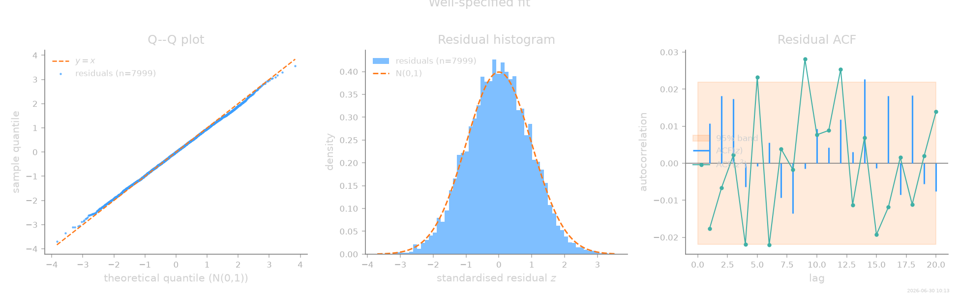
Text(0.5, 1.01, 'Well-specified fit')

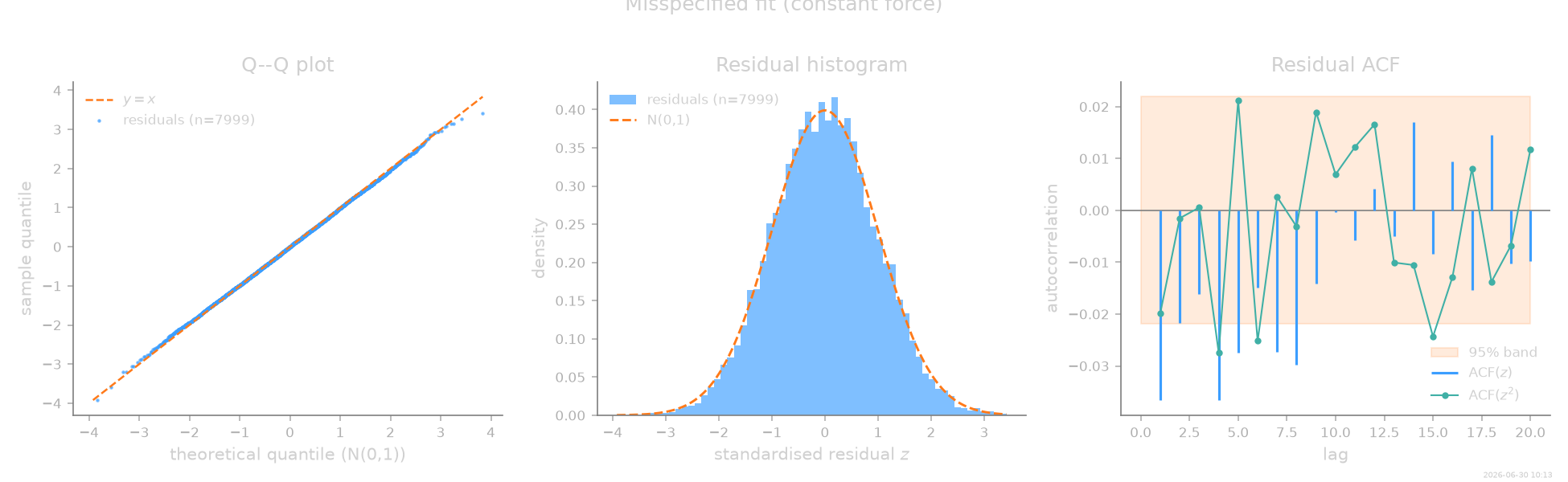
fig_bad = plot_summary(rep_bad)
fig_bad.suptitle("Misspecified fit (constant force)", y=1.01)

plt.show()

Reading the figures

The well-specified cubic fit shows residuals lining up on the Q–Q diagonal, a histogram that hugs the \(\mathcal N(0,1)\) density, and an ACF inside the Bartlett band; its printed report lists no flags.

The misspecified linear fit shows the diagnostic signature of a missing structural term: the leftover cubic force tracks the slow well-to-well motion, so the residuals are autocorrelated (the Ljung–Box test fails) and the realised NMSE sits well above the predicted (sampling-noise) value — the data does not support the linear model.

Note

How visible a missing term is depends on the sampling interval. At very fine \(\Delta t\) the diffusion estimate can absorb a weak force misspecification, leaving the marginal residual tests looking clean; coarser sampling (as here) makes the leftover structure show up in the autocorrelation and NMSE-consistency checks.

stamp_output()

[Generated: 2026-06-30 10:13]

🏷 Tags: diagnostics, overdamped, linear, 1D, synthetic