2D limit cycle — nonlinear overdamped inference

Infer the force field of a 2D nonlinear system with a stable limit cycle. The radial force \(\dot{r} = r(1 - r^2)\) drives the system to a unit circle, while an angular drift \(\dot{\theta} = \omega\) generates rotation — a non-equilibrium steady state with non-zero probability currents.

Tags

synthetic · overdamped · nonlinear · non-equilibrium · 2D

System definition

In Cartesian coordinates the force is:

\[F_x = x(1 - x^2 - y^2) - \omega\, y, \qquad F_y = y(1 - x^2 - y^2) + \omega\, x\]

with angular frequency \(\omega = 2\) and isotropic noise \(D = 0.1\).

from SFI.bases import named_scalars, ones_basis, unit_axes, x_components
from SFI.langevin import OverdampedProcess

# Ground-truth force written compositionally:
#     F = (1 - r^2) (x e_x + y e_y) + omega (x e_y - y e_x)
# with r^2 = x^2 + y^2.  ``named_scalars`` holds ``omega`` with a
# default value so the simulator can bind parameters automatically.
x, y = x_components(2)
ex, ey = unit_axes(2)
one = ones_basis(2)
(omega_p,) = named_scalars(omega=2.0)

r2 = x * x + y * y
F_true = (one - r2) * (x * ex + y * ey) + omega_p * (x * ey - y * ex)

D0 = 0.1
dt = 0.05
Nsteps = 4_000
seed = 0

proc = OverdampedProcess(F_true, D=jnp.eye(2) * D0)
proc.initialize(jnp.array([0.5, 0.0]))

key = random.PRNGKey(seed)
coll = proc.simulate(dt=dt, Nsteps=Nsteps, key=key, prerun=5000, oversampling=20)

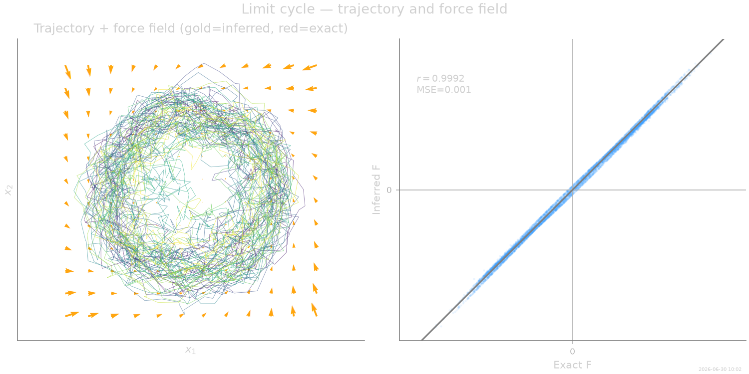
Trajectory and inferred force field

Build a polynomial basis, infer, sparsify with PASTIS, then overlay the inferred force field on the trajectory.

from SFI.bases import monomials_up_to
from SFI import OverdampedLangevinInference
from SFI.utils import plotting

degree = 3
B = monomials_up_to(order=degree, dim=2, include_constant=True, rank='vector')

inf = OverdampedLangevinInference(coll)
inf.compute_diffusion_constant()
inf.infer_force_linear(B, M_mode="Ito")
inf.compute_force_error()

inf.sparsify_force(criterion="PASTIS")
inf.compare_to_exact(model_exact=proc, maxpoints=2000)

inf.print_report()

  --- StochasticForceInference Report ---
Average diffusion tensor:
 [[ 0.1006882  -0.0014048 ]
 [-0.0014048   0.10216548]]
Measurement noise tensor:
 [[-0.00485671 -0.00024895]
 [-0.00024895 -0.00476173]]
Force estimated information: 2099.39599609375
Force: estimated normalized mean squared error (sampling only): 0.0047632734165367506
Normalized MSE (force):     0.0017
Normalized MSE (diffusion): 0.0004

  Force Coefficient Table
  ─────────────────────────────────────────────────────────────────────
  #    Label          Coefficient       Std.Err     SNR  Sig
  ─────────────────────────────────────────────────────────────────────
  2    x0·e0          1.13881e+00   1.45951e-01     7.8  *
  3    x0·e1          2.03314e+00   1.47018e-01    13.8  **
  4    x1·e0         -1.94517e+00   1.38036e-01    14.1  **
  5    x1·e1          9.05424e-01   1.39045e-01     6.5  *
  12   x0^3·e0       -1.02404e+00   1.19558e-01     8.6  *
  15   (x0^2·x1)·e1  -1.03951e+00   1.52876e-01     6.8  *
  16   (x0·x1^2)·e0  -1.14151e+00   1.55510e-01     7.3  *
  19   x1^3·e1       -9.12634e-01   1.12635e-01     8.1  *
  ─────────────────────────────────────────────────────────────────────
  8/20 basis functions in support, sig: 8* / 2** / 0*** (|SNR| ≥ 2 / 10 / 100)
  (Std.err. reflects sampling error only; discretization bias is not included.)
  Zeroed (12): 1·e0, 1·e1, x0^2·e0, x0^2·e1, (x0·x1)·e0, (x0·x1)·e1, x1^2·e0, x1^2·e1, x0^3·e1, (x0^2·x1)·e0, (x0·x1^2)·e1, x1^3·e0

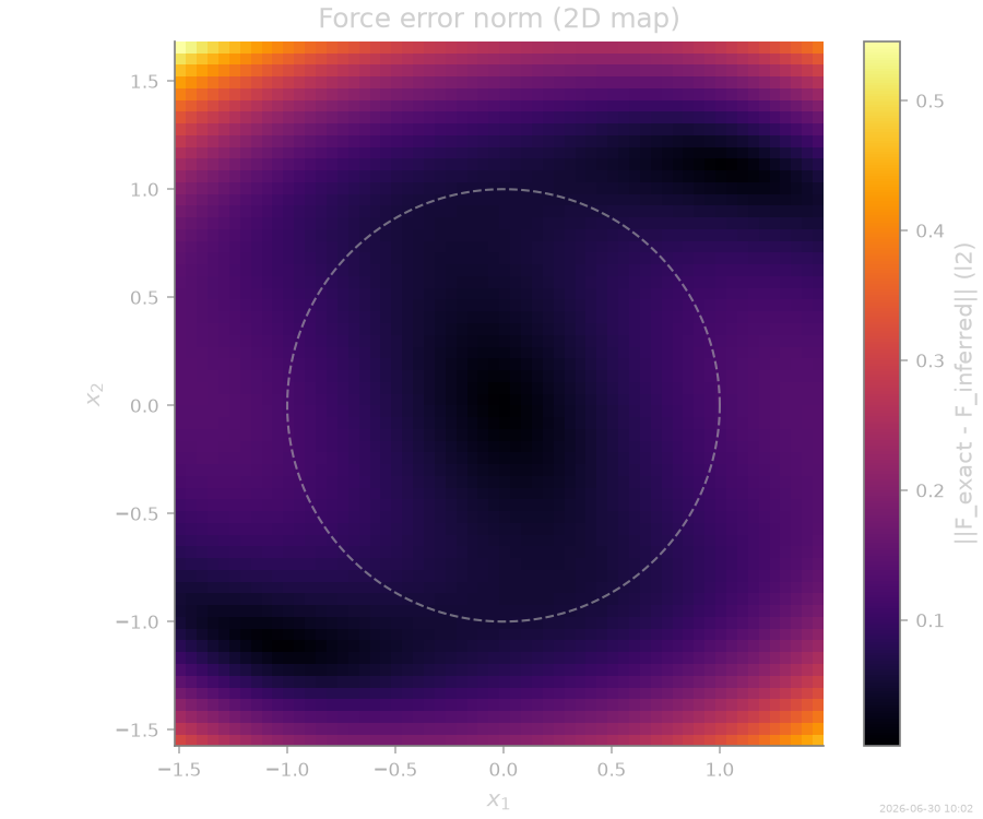
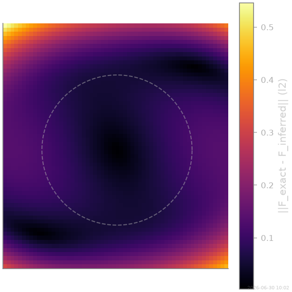
Force error norm

A 2D map of the force-reconstruction error \(\|F_{\mathrm{exact}} - F_{\mathrm{inferred}}\|\) evaluated on a regular grid covering the data domain.

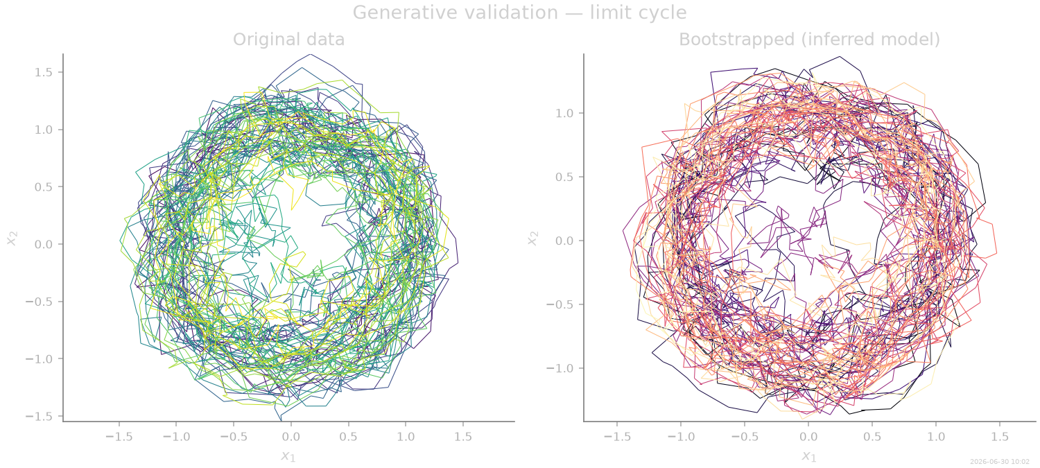
Bootstrapped trajectory

A trajectory simulated from the inferred model should reproduce the limit-cycle structure and rotational dynamics.

key_boot = random.PRNGKey(seed + 123)
coll_boot, _ = inf.simulate_bootstrapped_trajectory(key_boot, oversampling=20)

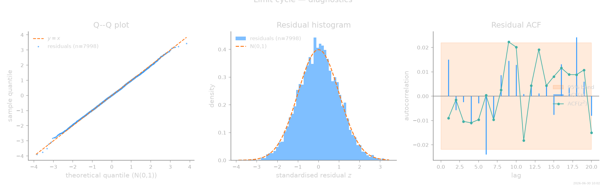
Diagnostics

assess() recomputes standardised residuals and runs a panel of consistency tests; a well-specified fit yields residuals consistent with i.i.d. \(\mathcal{N}(0, 1)\) — no autocorrelation, no excess kurtosis, and a realised NMSE consistent with the predicted value.

from SFI.diagnostics import assess, plot_summary

report = assess(inf, level="standard")
report.print_summary()

=== SFI diagnostics report ===
backend  : linear
regime   : OD
n_obs    : 3999  n_particles: 1  d: 2
level    : standard

-- Residuals --
  mean = +0.0133  std = 0.9777  skew = +0.007  kurt-3 = +0.010  (n=7998)
  ✓ normality ks                 stat=0.0136    p=0.103
  ✓ autocorr  ljung_box          stat=20        p=0.456
  ✓ autocorr  ljung_box_squared  stat=22.7      p=0.303
  predicted NMSE = 0.00476  realised NMSE = 0  χ² z = -2.78 (|z|>5 ⇒ bias)

-- Flags --
  (no issues at α = 0.01)

Thumbnail

Compact force-error map for the gallery grid.

stamp_output()

[Generated: 2026-06-30 10:02]

🏷 Tags: synthetic, overdamped, nonlinear, non-equilibrium, 2D