Velocity-dependent noise — underdamped multiplicative diffusion

Recover a velocity-dependent diffusion field \(D(v)\) for an inertial particle, from positions only. Many active and driven systems fluctuate harder the faster they move — motility noise, flight-force fluctuations, turbulent drag. Underdamped SFI reconstructs the unobserved velocity and infers \(F(x,v)\) and \(D(x,v)\) jointly; here the noise amplitude doubles within the explored speed range and is recovered model-free.

Tags

synthetic · underdamped · multiplicative-noise · diffusion-field · 1D

Model and simulation

A damped harmonic oscillator whose bath kicks grow with speed:

\[\dot x = v, \qquad dv = (-k x - \gamma v)\,dt + \sqrt{2 D(v)}\,dW, \qquad D(v) = D_0\left(1 + (v/v_c)^2\right),\]

in the Itô convention: the force SFI infers is the Itô drift of the velocity equation. Both fields are composed from coordinate primitives — note the velocity primitive v entering the diffusion.

import SFI
from SFI.bases import identity_matrix_basis, unit_axes, v_components, x_components
from SFI.langevin import UnderdampedProcess

k = 1.0       # stiffness
gamma = 1.0   # friction
D0 = 0.3      # diffusion at rest
vc = 1.0      # velocity scale of the noise growth
dt = 0.01
Nsteps = 80_000

(x,) = x_components(1)
(v,) = v_components(1)
(ex,) = unit_axes(1)
I = identity_matrix_basis(1)

F_model = (-k * x - gamma * v) * ex            # Itô drift of dv
D_model = D0 * (1.0 + (v / vc) ** 2) * I       # D(v) — multiplicative in v

proc = UnderdampedProcess(F=F_model, D=D_model,
                          theta_F=jnp.ones(F_model.n_features),
                          theta_D=jnp.ones(D_model.n_features))
proc.initialize(jnp.array([0.0]), v0=jnp.array([0.0]))
coll = proc.simulate(dt=dt, Nsteps=Nsteps, key=random.PRNGKey(5),
                     prerun=500, oversampling=20)
print(f"Trajectory: {coll.T} frames, dt={dt} (positions only)")

Trajectory: 80000 frames, dt=0.01 (positions only)

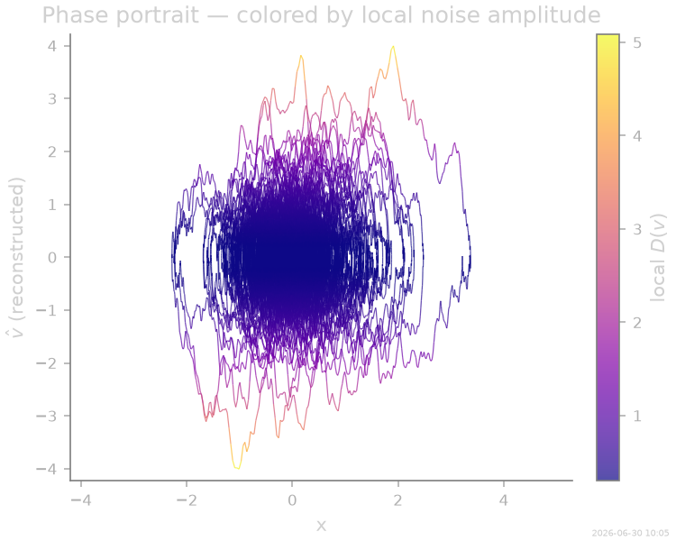
Phase portrait

Velocity is not observed — for plotting we reconstruct it by finite differences, exactly as the inference engine does internally. Fast excursions (top and bottom) are noticeably noisier than slow ones.

Inference

The underdamped parametric sequence: infer_force() fits the Itô drift \(F(x,v)\), then infer_diffusion() fits \(D(x,v)\) on a polynomial basis in both variables (include_v=True). The basis spans \(\{1, x, v, x^2, xv, v^2\}\) — the inference must discover that only \(1\) and \(v^2\) carry weight.

from SFI.bases import monomials_up_to

B_force = monomials_up_to(order=1, dim=1, include_v=True, rank="vector")
B_diff = monomials_up_to(order=2, dim=1, include_v=True, rank="symmetric_matrix")

inf = SFI.UnderdampedLangevinInference(coll)
inf.infer_force(B_force)
inf.infer_diffusion(B_diff)

inf.compare_to_exact(model_exact=proc)
inf.print_report()
print(inf.summary(field="diffusion"))
print(f"  (true: [1] = {D0:+.3f}, [v²] = {D0 / vc**2:+.3f}, rest 0)")

  --- StochasticForceInference Report ---
Average diffusion tensor:
 [[0.41754755]]
Measurement noise tensor:
 [[4.550176e-10]]
Normalized MSE (force):     0.0051
Normalized MSE (diffusion): 0.0003

  Force Coefficient Table
  ──────────────────────────────────────
  #    Label   Coefficient  Sig
  ──────────────────────────────────────
  0    b0      1.79458e-02  ·
  1    b1     -9.22756e-01  ·
  2    b2     -1.05463e+00  ·
  ──────────────────────────────────────
  3/3 basis functions in support
  Diffusion Coefficient Table
  ──────────────────────────────────────
  #    Label   Coefficient  Sig
  ──────────────────────────────────────
  0    b0      2.93479e-01  ·
  1    b1     -3.04928e-03  ·
  2    b2     -3.01497e-03  ·
  3    b3      3.06650e-03  ·
  4    b4      3.53166e-03  ·
  5    b5      3.07988e-01  ·
  ──────────────────────────────────────
  6/6 basis functions in support
  (true: [1] = +0.300, [v²] = +0.300, rest 0)

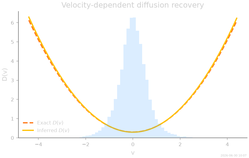
Recovered diffusion profile

Evaluating the inferred tensor along the velocity axis recovers the parabolic noise profile; a constant-\(D\) analysis would report only the mean.

# The inferred tensor as a callable on phase-space points [x, v]; sweeping the
# v axis (x held at 0) recovers the parabolic noise profile.
def D_inferred(pts):
    pts = jnp.asarray(pts)
    return inf.diffusion_inferred(pts[:, :1], v=pts[:, 1:2])  # (N, 1, 1)


def D_exact(pts):
    v = np.asarray(pts)[:, 1]
    return D0 * (1 + (v / vc) ** 2)

When is this hard?

Velocity-dependent noise has a genuinely hard regime. With \(D(v) \propto v^2\) the velocity distribution develops power-law tails (tail exponent \(2 + \gamma/D_0\)): if friction is weak relative to the noise gradient, rare high-speed bursts dominate the statistics, and no finite sampling rate resolves them — estimates of the noise floor \(D_0\) then degrade no matter how small \(dt\) is. Here \(\gamma/D_0 \approx 3.3\) keeps the tails integrable and the inference quantitative. For strongly driven systems, prefer saturating noise models (e.g. \(D_0 + \Delta D\, v^2/(v^2 + v_s^2)\)) — see the state-dependent diffusion benchmark for that case.

Thumbnail

Dedicated single-panel figure for the gallery thumbnail.

stamp_output()

[Generated: 2026-06-30 10:07]

🏷 Tags: synthetic, underdamped, multiplicative-noise, diffusion-field, 1D