Note
Go to the end to download the full example code.
Multiplicative noise — the Landauer blowtorch
Recover a state-dependent diffusion field \(D(x)\) together with the force from a single overdamped trajectory. The system is the classic Landauer blowtorch: a bistable particle whose bath is hotter on one side. The temperature gradient redistributes the well occupancies away from the naive Boltzmann weights — an effect that only a joint inference of \(F(x)\) and \(D(x)\) can capture.
Tags
synthetic · overdamped · multiplicative-noise · diffusion-field · 1D
Model and simulation
A double-well particle in a bath with a linear temperature profile:
interpreted in the Itô convention — the drift entering the SDE
(and the force SFI infers) is the Itô drift. With \(g > 0\) the
right well sits in the hot region. Both fields are built
compositionally from SFI.bases primitives and passed straight
to the simulator.
import SFI
from SFI.bases import identity_matrix_basis, unit_axes, x_components
from SFI.langevin import OverdampedProcess

D0 = 0.5      # baseline diffusion
g = 0.3       # temperature gradient
dt = 0.01
Nsteps = 50_000

(x,) = x_components(1)
(ex,) = unit_axes(1)
I = identity_matrix_basis(1)

F_model = (x - x**3) * ex                # F(x) = x - x³  (Itô drift)
D_model = D0 * (1.0 + g * x) * I         # D(x) = D₀(1 + g·x)

proc = OverdampedProcess(F=F_model, D=D_model,
                         theta_F=jnp.array([1.0]), theta_D=jnp.array([1.0]))
proc.initialize(jnp.array([0.5]))
coll = proc.simulate(dt=dt, Nsteps=Nsteps, key=random.PRNGKey(7),
                     prerun=200, oversampling=10)
print(f"Trajectory: {coll.T} frames, dt={dt}")
Trajectory: 50000 frames, dt=0.01
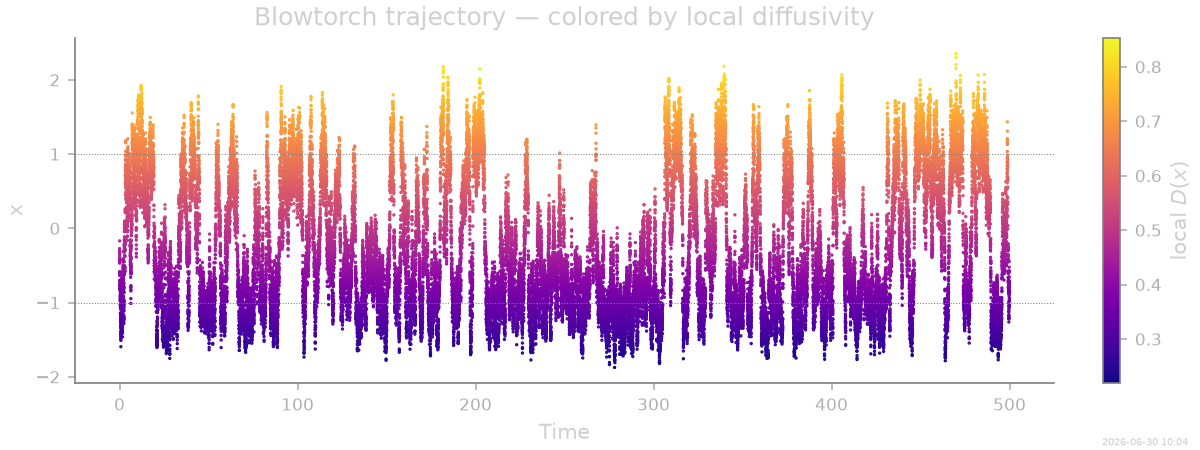
Trajectory
The particle hops between the two wells; excursions in the hot (right) well are visibly more agitated than in the cold one.
Inference: force, then diffusion field
The linear-estimator sequence, with one extra step: after the usual
constant-\(D\) estimate and force regression, we fit the full
diffusion field with infer_diffusion_linear() on a rank-2
polynomial basis (rank='symmetric_matrix'). The quadratic basis
is deliberately larger than the truth — the linear gradient must be
discovered, not assumed.
from SFI.bases import monomials_up_to

B_force = monomials_up_to(order=3, dim=1, rank="vector")
B_diff = monomials_up_to(order=2, dim=1, rank="symmetric_matrix")

inf = SFI.OverdampedLangevinInference(coll)
inf.compute_diffusion_constant()              # constant-D baseline
inf.infer_force_linear(B_force)               # Itô drift regression
inf.compute_force_error()
inf.infer_diffusion_linear(B_diff)            # state-dependent D(x)

inf.compare_to_exact(model_exact=proc)
inf.print_report()
  --- StochasticForceInference Report ---
Average diffusion tensor:
 [[0.4486813]]
Measurement noise tensor:
 [[4.6545298e-05]]
Force estimated information: 201.67665100097656
Force: estimated normalized mean squared error (sampling only): 0.009916864396911845
Normalized MSE (force):     0.0256
Normalized MSE (diffusion): 0.0014

  Force Coefficient Table
  ────────────────────────────────────────────────────────────────
  #    Label     Coefficient       Std.Err     SNR  Sig
  ────────────────────────────────────────────────────────────────
  0    1·e0     -1.36633e-02   6.81399e-02     0.2  ·
  1    x0·e0     9.64689e-01   1.08198e-01     8.9  *
  2    x0^2·e0  -7.86582e-02   6.18999e-02     1.3  ·
  3    x0^3·e0  -1.06802e+00   6.65354e-02    16.1  **
  ────────────────────────────────────────────────────────────────
  4/4 basis functions in support, sig: 2* / 1** / 0*** (|SNR| ≥ 2 / 10 / 100)
  (Std.err. reflects sampling error only; discretization bias is not included.)
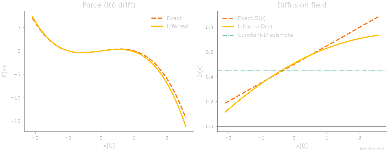
Recovered force and diffusion fields
Both fields are recovered from the same trajectory. The constant-D baseline (what a standard analysis would report) misses the gradient entirely.
x_grid = np.linspace(-1.9, 1.9, 200)
x_jnp = jnp.array(x_grid[:, None])
F_exact = x_grid - x_grid**3
D_exact = D0 * (1 + g * x_grid)
F_inf = np.asarray(inf.force_inferred(x_jnp))[:, 0]
D_inf = np.asarray(inf.diffusion_inferred(x_jnp))[:, 0, 0]
D_const = float(np.asarray(inf.diffusion_average).ravel()[0])
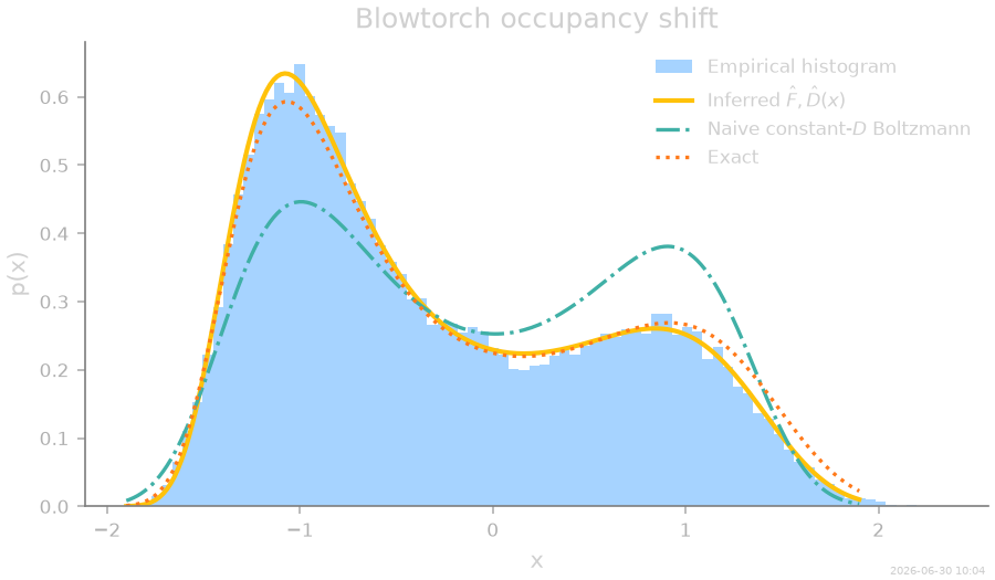
The blowtorch effect: occupancy statistics
For Itô dynamics the zero-current stationary density is
not the Boltzmann weight \(e^{-U(x)/\bar D}\) built from the potential and a constant diffusion estimate. The hot well is depopulated. Using the inferred \(\hat F\) and \(\hat D(x)\) in the formula above reproduces the empirical histogram; the constant-D Boltzmann prediction does not.
from scipy.integrate import cumulative_trapezoid


def stationary_density(F_vals, D_vals, x_vals):
    """Zero-current Itô stationary density on a grid (unnormalized)."""
    phi = cumulative_trapezoid(F_vals / D_vals, x_vals, initial=0.0)
    p = np.exp(phi - phi.max()) / D_vals
    return p / np.trapezoid(p, x_vals)


p_exact = stationary_density(F_exact, D_exact, x_grid)
p_inferred = stationary_density(F_inf, D_inf, x_grid)
p_naive = stationary_density(F_inf, np.full_like(x_grid, D_const), x_grid)
A note on spurious drifts
With multiplicative noise the words “force” and “drift” need care. SFI infers the Itô drift \(F\): the conditional mean displacement per unit time, \(F(x) = \lim_{dt\to 0} \langle \Delta x \rangle / dt\). Other stochastic conventions absorb part of the noise gradient into the drift — in 1D,
and these spurious drift terms have real dynamical consequences: even with zero force, Itô dynamics accumulates particles in low-noise regions (\(p \propto 1/D\)), so a bare drift measurement can suggest a force toward the cold side where none exists. Whether the physical system at hand obeys Itô, Stratonovich or isothermal (anti-Itô) statistics is an experimental question — but once \(F_{\rm Itô}\) and \(D(x)\) are both inferred, converting between conventions is just the dictionary above.
Thumbnail
Dedicated single-panel figure for the gallery thumbnail.
stamp_output()

[Generated: 2026-06-30 10:04]
Total running time of the script: (0 minutes 15.839 seconds)