Time-dependent forcing — protocols as extras

Infer a force law that depends on a known time-dependent protocol — here a trap whose stiffness is switched between two values — from a single 1D trajectory.

The protocol \(k(t)\) enters SFI as a time-dependent extra: the simulator consumes it per frame, attaches it to the output collection, and the inference reads it back through the compositional symbol extra_scalar(). The same mechanism covers temperature ramps, oscillating fields, or any drive recorded alongside the trajectory.

Tags

synthetic · overdamped · linear · 1D · time-dependent

Model: a trap with switched stiffness

An overdamped particle in a harmonic trap whose stiffness alternates between two plateaus:

\[dx = -\bigl[k_0 + k(t)\bigr]\,x\,dt + \sqrt{2D}\,dW,\]

with \(k_0 = 1\), a square-wave drive \(k(t) \in \{0, 1\}\), and \(D = 0.25\). The force model is built compositionally: the drive is a basis symbol read from the dataset’s extras.

import SFI
from SFI.bases import X, extra_scalar
from SFI.langevin import OverdampedProcess
from SFI.trajectory import time_series_extra

dt = 0.01
Nsteps = 20_000
period = 1_000  # frames per plateau

k_protocol = (np.arange(Nsteps) // period % 2).astype(float)

# Two-feature basis: static trap x, and protocol-modulated trap k(t)·x.
B = X(dim=1) & (extra_scalar("k_drive", dim=1) * X(dim=1))

proc = OverdampedProcess(F=B, D=0.25, theta_F=jnp.array([-1.0, -1.0]))
proc.set_extras(extras_global={"k_drive": time_series_extra(k_protocol)})
proc.initialize(jnp.zeros(1))

coll = proc.simulate(dt=dt, Nsteps=Nsteps, key=random.PRNGKey(42), oversampling=4)

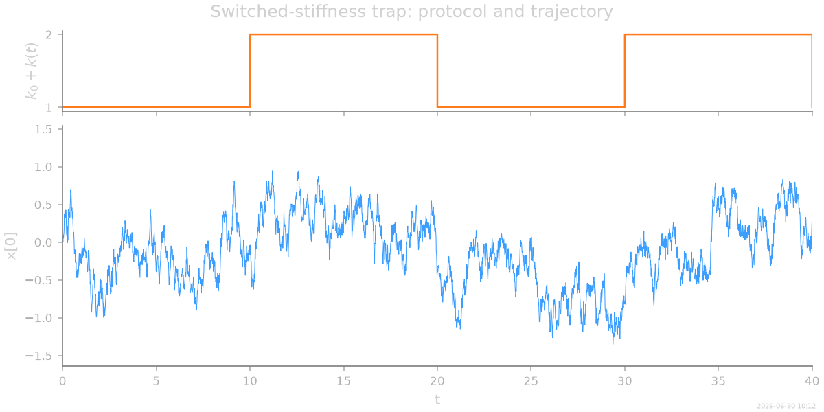
Trajectory and protocol

When the drive is on, the trap is twice as stiff and the fluctuations shrink accordingly.

Inference with the protocol as a basis symbol

The same two-feature dictionary serves for inference: the linear estimator reads k_drive per frame from the collection’s extras (the simulator attached it), so the static and driven contributions are separated by the protocol’s variation.

inf = SFI.OverdampedLangevinInference(coll)
inf.compute_diffusion_constant()
inf.infer_force_linear(B)
inf.compute_force_error()
inf.print_report()

  --- StochasticForceInference Report ---
Average diffusion tensor:
 [[0.24711466]]
Measurement noise tensor:
 [[2.6887963e-05]]
Force estimated information: 71.08001708984375
Force: estimated normalized mean squared error (sampling only): 0.014068653331150848

  Force Coefficient Table
  ──────────────────────────────────────────────────────────────────
  #    Label       Coefficient       Std.Err     SNR  Sig
  ──────────────────────────────────────────────────────────────────
  0    x          -1.04602e+00   1.44900e-01     7.2  *
  1    k_drive·x  -7.57706e-01   2.39010e-01     3.2  *
  ──────────────────────────────────────────────────────────────────
  2/2 basis functions in support, sig: 2* / 0** / 0*** (|SNR| ≥ 2 / 10 / 100)
  (Std.err. reflects sampling error only; discretization bias is not included.)

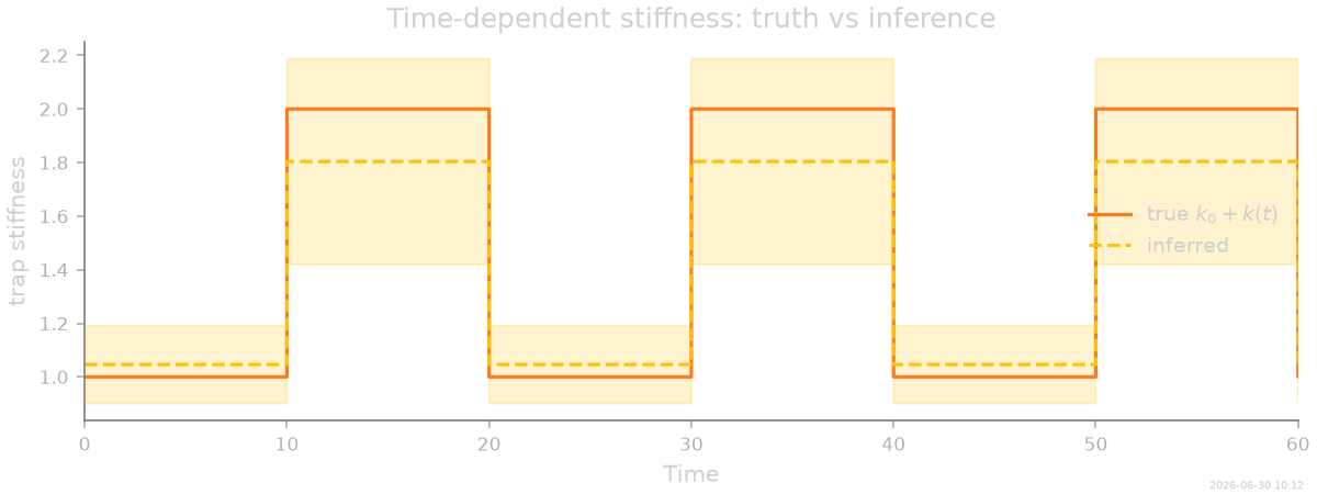
Recovered stiffness law

The two fitted coefficients reconstruct the time-dependent stiffness \(\hat k(t) = -[\hat\theta_1 + \hat\theta_2\,k(t)]\), compared to the ground truth.

Notes

• In simulation, set_extras accepts a TimeSeriesExtra (one value per recorded frame, held across oversampling substeps) or a plain callable f(t) of physical time; the schedule is attached to the returned collection.

• In inference, any time-dependent extra in the dataset is sliced per frame automatically; extra_scalar() turns it into a composable basis symbol.

• The static and driven features are collinear up to the protocol’s variation — strongly varying protocols (switches, large ramps) identify the split best, and force_coefficients_stderr reports exactly how well.

stamp_output()

[Generated: 2026-06-30 10:12]

🏷 Tags: synthetic, overdamped, linear, 1D, time-dependent