Gray-Scott reaction-diffusion: SPDE inference

Note

Uses the experimental SPDE toolbox — see SPDE (spatial fields) — experimental.

Infer the reaction-diffusion dynamics of a stochastic Gray-Scott system on a 2D grid. This demonstrates SFI’s SPDE capabilities:

• GridLayout composing differential operators on named field sectors: layout.lap(U) applies a 5-point Laplacian stencil to the U sector, layout.grad(U).dot(layout.grad(V)) builds cross-gradient features, and layout.embed(rank=1, ...) compiles everything into a single force model

• Auto-generated feature labels from the expression tree, using with_label() and operator auto-labelling

• PASTIS sparsification recovering the exact 7-term model from a 34-feature over-specified basis (all order-3 monomials, Laplacians, gradient products, and biharmonics)

• Conserved noise — conserved_noise_pbc() provides \(\nabla\!\cdot\!\boldsymbol\eta\) noise whose spatial average is exactly zero at every time step

• Overdamped inference on high-dimensional state spaces

• Degradation of spatial data and bootstrap validation

• Multi-regime robustness — the same basis recovers the same 7-term structure across distinct \((F, K)\) regimes

The Gray-Scott model defines two interacting fields \(U, V\) with conserved (divergence-form) stochastic transport:

\[ \begin{align}\begin{aligned}\dot{U} = D_U \nabla^2 U - U V^2 + F (1-U) + \sigma\,\nabla\!\cdot\!\boldsymbol\eta_U\\\dot{V} = D_V \nabla^2 V + U V^2 - (F+K) V + \sigma\,\nabla\!\cdot\!\boldsymbol\eta_V\end{aligned}\end{align} \]

where \(\boldsymbol\eta_{U,V}\) are independent spatiotemporal white vector noises. The conserved noise ensures that any spatial average \(\langle U \rangle, \langle V \rangle\) changes only through the deterministic dynamics, not through noise.

Tags

synthetic · overdamped · SPDE · reaction-diffusion · 2D · sparsification · multi-experiment

System setup

We use a 64×64 grid with dx = 1 (physical domain \(L = 64\)). The Turing wavelength \(\lambda \approx 2\pi\sqrt{D_U/F} \approx 12\) fits about five times across the domain, giving well-developed patterns. Inference is local — it fits the finite-difference stencil at every cell — so the 4096 cells supply ample constraints for the operators.

The force model is built with GridLayout: two named ScalarSector fields U and V share a single layout. Differential operators (layout.lap) and pointwise algebra (U * V * V) compose freely; layout.embed compiles the whole expression tree into an inference-ready Basis.

from SFI.bases.spde import conserved_noise_pbc, square_grid_extras
from SFI.langevin import OverdampedProcess
from SFI.statefunc.layout import GridLayout, ScalarSector

DIM = 2  # field dimension (U, V)
GRID = (64, 64)
DT = 0.5
DX = 1.0
STEPS = 500
OVERS = 4
PRERUN = 200   # burn-in frames: let patterns develop before recording
SEED = 0

# Gray-Scott parameters — "coral" regime
DU, DV = 0.16, 0.08
F_gs, K_gs = 0.042, 0.063

# Conserved noise amplitude (same for both fields)
SIGMA = 0.01

# --- GridLayout: two scalar sectors on a 2D periodic grid ---
layout = GridLayout(
    U=ScalarSector([0]),
    V=ScalarSector([1]),
    dim=DIM, ndim=2, bc="pbc",
)
U = layout.U   # StructuredExpr for U field
V = layout.V   # StructuredExpr for V field

Over-specified basis

Rather than hand-coding the exact 7-term Gray-Scott structure, we build a generic basis: all monomials up to order 3 in \((U, V)\), differential operators \(\nabla^2, \nabla^4\), and nonlinear gradient terms \(|\nabla U|^2, |\nabla V|^2, \nabla U \cdot \nabla V\). This gives 17 candidate features per channel = 34 total. PASTIS will prune this down to the correct 7.

Labels are generated automatically from the expression tree — each single-feature term carries its own human-readable string via operator auto-labelling (e.g. U ** 2 → "U²", layout.lap(U) → "∇²U", gU.dot(gV) → "∇U·∇V").

ONE = layout.const(1)                 # auto: "1"
gU = layout.grad(U)
gV = layout.grad(V)

terms = [
    # --- pointwise monomials ---
    ONE,                              # auto: "1"
    U, V,                             # auto: "U", "V"
    U**2, U * V, V**2,               # auto: "U²", "UV", "V²"
    U**3, U**2 * V, U * V**2, V**3,  # auto: "U³", "U²V", "UV²", "V³"
    # --- Laplacian ---
    layout.lap(U),                    # auto: "∇²U"
    layout.lap(V),                    # auto: "∇²V"
    # --- gradient product terms ---
    gU.dot(gU),                       # auto: "∇U·∇U"
    gV.dot(gV),                       # auto: "∇V·∇V"
    gU.dot(gV),                       # auto: "∇U·∇V"
    # --- biharmonic ---
    layout.biharmonic(U),             # auto: "∇⁴U"
    layout.biharmonic(V),             # auto: "∇⁴V"
]

# Concatenate features using &
generic = terms[0]
for t in terms[1:]:
    generic = generic & t

# Same candidate set for both channels
BASIS = layout.embed(rank=1, U=generic, V=generic)

# Labels are auto-derived from the expression tree
auto_labels = list(generic.labels)
n_per = len(auto_labels)   # 17
n_feat = 2 * n_per         # 34
labels = [f"{lbl}→U̇" for lbl in auto_labels] + \
         [f"{lbl}→V̇" for lbl in auto_labels]

# Ground truth: 7 non-zero out of 34
#   U channel (indices 0–16):  F·1, −F·U, −1·UV², D_U·∇²U
#   V channel (indices 17–33): +1·UV², −(F+K)·V, D_V·∇²V
theta_dense = np.zeros(n_feat)
theta_dense[0] = F_gs             # 1→U̇
theta_dense[1] = -F_gs            # U→U̇
theta_dense[8] = -1.0             # UV²→U̇
theta_dense[10] = DU              # ∇²U→U̇
theta_dense[n_per + 8] = +1.0     # UV²→V̇
theta_dense[n_per + 2] = -(F_gs + K_gs)  # V→V̇
theta_dense[n_per + 11] = DV      # ∇²V→V̇

support_true = list(np.nonzero(theta_dense)[0])
coeffs_true = theta_dense[support_true]

theta_sim = jnp.array(theta_dense, dtype=jnp.float32)

Simulate with burn-in

A prerun of 200 frames (100 time units) lets the Turing pattern develop from the initial seed before we start recording. This improves inference quality because the data covers the developed attractor rather than a featureless transient.

noise = conserved_noise_pbc(sigma=SIGMA, grid_shape=GRID, dx=DX, n_fields=DIM)
box_extras = square_grid_extras(grid_shape=GRID, dx=DX)

# Initial condition (symmetry-broken seed in the centre)
Nx, Ny = GRID
U0 = jnp.ones((Nx, Ny), dtype=jnp.float32)
V0 = jnp.zeros((Nx, Ny), dtype=jnp.float32)
r = min(Nx, Ny) // 8
cx, cy = Nx // 2, Ny // 2
U0 = U0.at[cx - r:cx + r, cy - r:cy + r].set(0.50)
V0 = V0.at[cx - r:cx + r, cy - r:cy + r].set(0.25)

key = random.PRNGKey(SEED)
key, sub = random.split(key)
U0 = U0 + 0.02 * random.normal(sub, U0.shape, dtype=U0.dtype)
key, sub = random.split(key)
V0 = V0 + 0.02 * random.normal(sub, V0.shape, dtype=V0.dtype)

X0 = jnp.stack([U0, V0], axis=-1).reshape((Nx * Ny, DIM))

proc = OverdampedProcess(BASIS, D=noise)
proc.set_params(theta_F=theta_sim)
proc.set_extras(extras_global=box_extras)
proc.initialize(X0)

key, sub = random.split(key)
t0 = time.perf_counter()
coll = proc.simulate(
    dt=DT, Nsteps=STEPS, key=sub, prerun=PRERUN, oversampling=OVERS,
)
elapsed = time.perf_counter() - t0
print(f"Simulation: {coll.T} frames, prerun={PRERUN}  "
      f"({elapsed:.1f}s)")

Simulation: 500 frames, prerun=200  (14.6s)

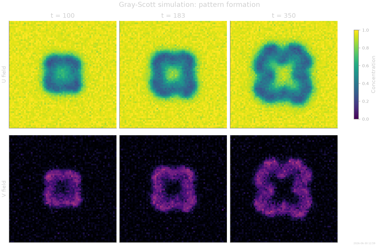
Simulated fields

Snapshots of the U and V fields after burn-in. By frame 0 the pattern is already developing; by the final frame the characteristic spot/labyrinth structure has emerged.

T_total = coll.T
snapshots = [0, T_total // 3, T_total - 1]

Degrade and infer

We introduce a small random pixel-loss fraction, mimicking missing data in experimental recordings. The 34-feature dense model is inferred first, before sparsification.

Note

Spatial coarsening (downscale > 1) is not applied here. For stencil-based operators like the Laplacian, down-sampling changes which neighbours the stencil sees; the coarse-grid Laplacian is a different finite-difference approximation from the fine-grid one that generated the data.

from SFI import OverdampedLangevinInference
from SFI.statefunc.nodes.interactions.prepare import purge_cache_extras
from SFI.trajectory.degrade import degrade_spatial_data

coll_deg = degrade_spatial_data(
    coll, downscale=1,
    data_loss_fraction=0.001, noise=0.0, bc="pbc",
)
coll_deg.extras_global = purge_cache_extras(coll_deg.extras_global)

inf = OverdampedLangevinInference(coll_deg)
inf.compute_diffusion_constant(method="WeakNoise")
inf.infer_force_linear(BASIS, M_mode="Ito")
inf.compute_force_error()

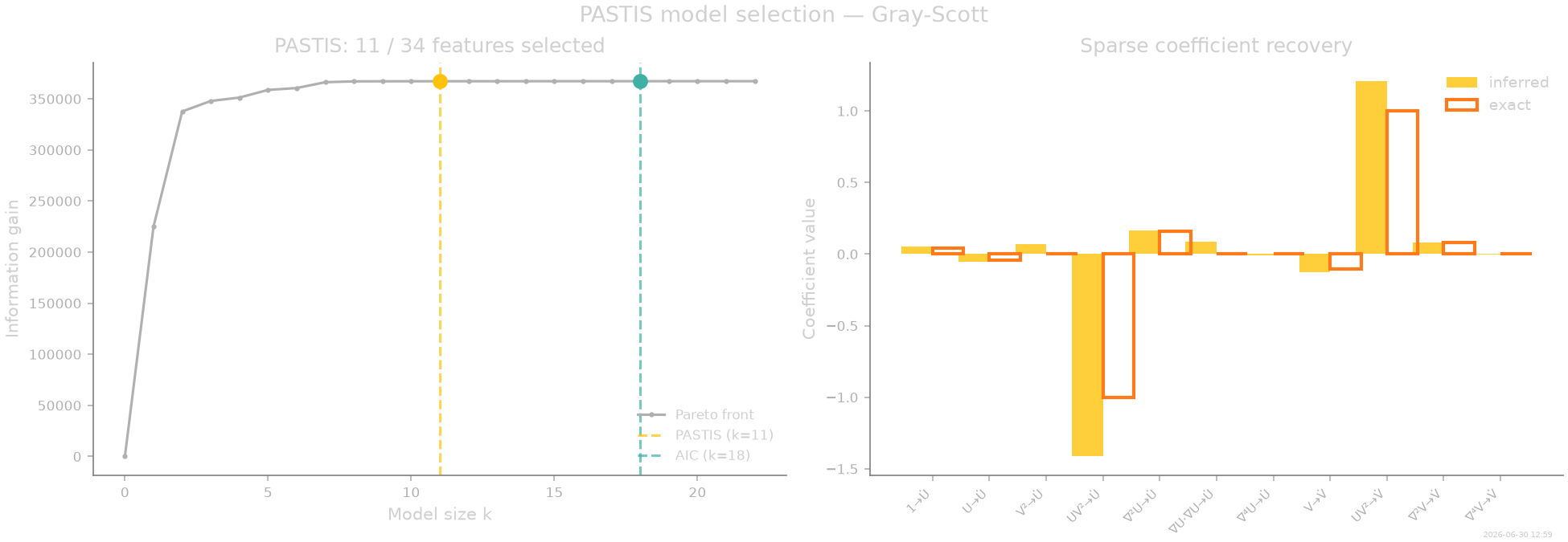
PASTIS sparsification

From the 34-feature dense solution, PASTIS selects the minimal model that passes the significance criterion. The 7 reaction-diffusion terms are always recovered; additionally, tiny biharmonic corrections (\(\nabla^4 U, \nabla^4 V\) with coefficients \(\sim 10^{-4}\)) may appear because the finite-difference Laplacian stencil introduces a small systematic \(O(dx^2)\) numerical artefact.

inf.sparsify_force(criterion="PASTIS", p=0.001)
inf.compute_force_error()
inf.compare_to_exact(model_exact=proc, maxpoints=30)

k_sel, support_sel, _, coeffs_sel = \
    inf.force_sparsity_result.select_by_ic("PASTIS")
print(f"True support recovered: {set(support_true).issubset(set(support_sel))}")

inf.print_report()

True support recovered: True

  --- StochasticForceInference Report ---
Average diffusion tensor:
 [[ 6.2343356e-04 -1.4497949e-06]
 [-1.4497949e-06  6.4761657e-04]]
Measurement noise tensor:
 [[9.0806738e-05 4.7643475e-06]
 [4.7643475e-06 5.8317470e-05]]
Force estimated information: 367245.46875
Force: estimated normalized mean squared error (sampling only): 1.497639930227704e-05
Normalized MSE (force):     0.0426

  Force Coefficient Table
  ──────────────────────────────────────────────────────────────
  #    Label   Coefficient       Std.Err     SNR  Sig
  ──────────────────────────────────────────────────────────────
  0    1       5.16088e-02   3.80596e-04   135.6  ***
  1    U      -5.16175e-02   3.99026e-04   129.4  ***
  5    V²      7.19335e-02   5.76799e-03    12.5  **
  8    UV²    -1.41341e+00   1.53800e-02    91.9  **
  10   ∇²U     1.65664e-01   1.06301e-03   155.8  ***
  12   ∇U·∇U   8.87408e-02   8.70039e-03    10.2  **
  15   ∇⁴U    -7.06458e-03   1.84601e-04    38.3  **
  19   V      -1.27887e-01   1.15641e-03   110.6  ***
  25   UV²     1.20779e+00   9.98330e-03   121.0  ***
  28   ∇²V     8.13759e-02   7.57109e-04   107.5  ***
  33   ∇⁴V    -1.61616e-03   1.26602e-04    12.8  **
  ──────────────────────────────────────────────────────────────
  11/34 basis functions in support, sig: 11* / 11** / 6*** (|SNR| ≥ 2 / 10 / 100)
  (Std.err. reflects sampling error only; discretization bias is not included.)
  Zeroed (23): V, U², UV, U³, U²V, V³, ∇²V, ∇V·∇V, ∇U·∇V, ∇⁴V, 1, U, U², UV, V², U³, U²V, V³, ∇²U, ∇U·∇U, ∇V·∇V, ∇U·∇V, ∇⁴U

Pareto front and sparse recovery

Left: information gain vs model size, with information-criterion thresholds. Right: inferred sparse coefficients overlaid on ground truth.

Coefficient comparison

print(model_summary(
    labels, np.array(coeffs_sel), support=support_sel,
    coeffs_true=coeffs_true, support_true=support_true,
    title="Gray-Scott sparse model: true vs inferred",
))

Gray-Scott sparse model: true vs inferred
────────────────────────────────────────────────────────
#    Label      Coefficient          True  Sig
────────────────────────────────────────────────────────
0    1→U̇       5.16088e-02   4.20000e-02  ·
1    U→U̇      -5.16175e-02  -4.20000e-02  ·
5    V²→U̇      7.19335e-02   0.00000e+00  ·
8    UV²→U̇    -1.41341e+00  -1.00000e+00  ·
10   ∇²U→U̇     1.65664e-01   1.60000e-01  ·
12   ∇U·∇U→U̇   8.87408e-02   0.00000e+00  ·
15   ∇⁴U→U̇    -7.06458e-03   0.00000e+00  ·
19   V→V̇      -1.27887e-01  -1.05000e-01  ·
25   UV²→V̇     1.20779e+00   1.00000e+00  ·
28   ∇²V→V̇     8.13759e-02   8.00000e-02  ·
33   ∇⁴V→V̇    -1.61616e-03   0.00000e+00  ·
────────────────────────────────────────────────────────
11/34 basis functions in support
Zeroed (23): V→U̇, U²→U̇, UV→U̇, U³→U̇, U²V→U̇, V³→U̇, ∇²V→U̇, ∇V·∇V→U̇, ∇U·∇V→U̇, ∇⁴V→U̇, 1→V̇, U→V̇, U²→V̇, UV→V̇, V²→V̇, U³→V̇, U²V→V̇, V³→V̇, ∇²U→V̇, ∇U·∇U→V̇, ∇V·∇V→V̇, ∇U·∇V→V̇, ∇⁴U→V̇

Bootstrap validation

Re-simulate from the inferred sparse model, starting from the first post-burn-in frame.

X0_boot = coll.X[0]  # post-burn-in initial condition

key, sub = random.split(key)
proc_boot = inf.simulate_bootstrapped_trajectory(sub, simulate=False)
proc_boot.set_extras(extras_global=box_extras)
proc_boot.initialize(X0_boot)

key, sub = random.split(key)
_boot_ok = False
for _boot_try in range(5):
    try:
        key, sub = random.split(key)
        coll_boot = proc_boot.simulate(
            dt=DT, Nsteps=STEPS, key=sub, prerun=0, oversampling=OVERS,
        )
        _boot_ok = True
        break
    except ValueError:
        print(f"  Bootstrap attempt {_boot_try + 1} diverged, retrying...")
if not _boot_ok:
    raise RuntimeError("Bootstrap diverged after 5 attempts")

ti_final = min(coll.T, coll_boot.T) - 1

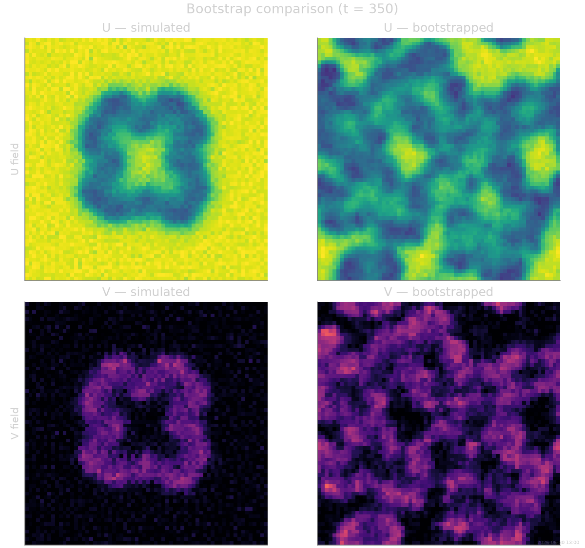
Side-by-side bootstrap movie

Animated comparison of original simulation (left) and bootstrap resimulation from the inferred sparse model (right). Both start from the same initial condition but evolve under independent noise realisations — the morphological statistics (spot density, ring thickness …) should match.

T_frames = min(coll.T, coll_boot.T)
skip_gs = max(1, T_frames // 150)

Multi-regime robustness

The 7-term reaction-diffusion structure should be recoverable across different \((F, K)\) regimes that produce visually distinct patterns. We re-run the simulate → degrade → infer → PASTIS pipeline on three regimes using the same over-specified basis, and check that PASTIS selects the same structural terms each time. The regime-independent coefficients (\(D_U\), \(D_V\), the \(\pm 1\) couplings) should stay fixed, while \(F\) and \((F{+}K)\) track the parameter change. The “Coral” entry reuses the fit from above.

def _true_theta(F, K):
    """The 7 non-zero coefficients for a given (F, K)."""
    th = np.zeros(n_feat)
    th[0] = F                       # 1   → U̇
    th[1] = -F                      # U   → U̇
    th[8] = -1.0                    # UV² → U̇
    th[10] = DU                     # ∇²U → U̇
    th[n_per + 8] = +1.0            # UV² → V̇
    th[n_per + 2] = -(F + K)        # V   → V̇
    th[n_per + 11] = DV             # ∇²V → V̇
    return th


def _seed_ic(key):
    """Symmetry-broken central seed, identical recipe to the main run."""
    U0r = jnp.ones((Nx, Ny), dtype=jnp.float32)
    V0r = jnp.zeros((Nx, Ny), dtype=jnp.float32)
    rr = min(Nx, Ny) // 8
    cxr, cyr = Nx // 2, Ny // 2
    U0r = U0r.at[cxr - rr:cxr + rr, cyr - rr:cyr + rr].set(0.50)
    V0r = V0r.at[cxr - rr:cxr + rr, cyr - rr:cyr + rr].set(0.25)
    k1, k2 = random.split(key)
    U0r = U0r + 0.02 * random.normal(k1, U0r.shape, dtype=U0r.dtype)
    V0r = V0r + 0.02 * random.normal(k2, V0r.shape, dtype=V0r.dtype)
    return jnp.stack([U0r, V0r], axis=-1).reshape((Nx * Ny, DIM))


# "Coral" is the regime fit above; add two more.
regimes = [("Spots", 0.030, 0.057), ("Coral", F_gs, K_gs), ("Holes", 0.050, 0.065)]
regime_results = {
    "Coral": dict(F=F_gs, K=K_gs, support=list(support_sel),
                  coeffs=np.array(coeffs_sel)),
}

for ri, (rname, Fr, Kr) in enumerate(regimes):
    if rname == "Coral":
        print(f"  {rname:>6} (F={Fr}, K={Kr}): reusing fit from above "
              f"({len(support_sel)} terms)")
        continue
    proc_r = OverdampedProcess(BASIS, D=noise)
    proc_r.set_params(theta_F=jnp.array(_true_theta(Fr, Kr), dtype=jnp.float32))
    proc_r.set_extras(extras_global=box_extras)
    key, sub_ic = random.split(key)
    proc_r.initialize(_seed_ic(sub_ic))
    key, sub = random.split(key)
    coll_r = proc_r.simulate(dt=DT, Nsteps=STEPS, key=sub,
                             prerun=PRERUN, oversampling=OVERS)
    coll_rd = degrade_spatial_data(
        coll_r, downscale=1, data_loss_fraction=0.001, noise=0.0, bc="pbc",
    )
    coll_rd.extras_global = purge_cache_extras(coll_rd.extras_global)
    inf_r = OverdampedLangevinInference(coll_rd)
    inf_r.compute_diffusion_constant(method="WeakNoise")
    inf_r.infer_force_linear(BASIS, M_mode="Ito")
    inf_r.compute_force_error()
    inf_r.sparsify_force(criterion="PASTIS", p=0.001)
    inf_r.compute_force_error()
    ks, sup_s, _, co_s = inf_r.force_sparsity_result.select_by_ic("PASTIS")
    regime_results[rname] = dict(F=Fr, K=Kr, support=list(sup_s),
                                 coeffs=np.array(co_s))
    print(f"  {rname:>6} (F={Fr}, K={Kr}): "
          f"true terms recovered = {set(support_true).issubset(set(sup_s))}")


def _coeff(res, idx):
    """Inferred coefficient at full-basis index idx (0 if pruned)."""
    return float(res["coeffs"][res["support"].index(idx)]) \
        if idx in res["support"] else 0.0

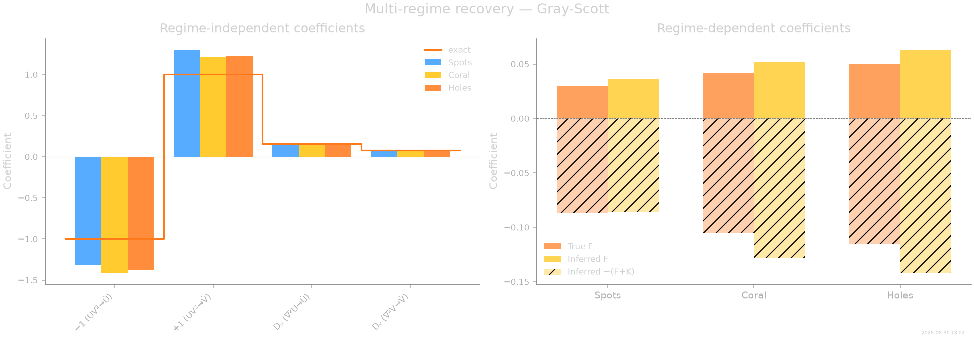
Spots (F=0.03, K=0.057): true terms recovered = True
Coral (F=0.042, K=0.063): reusing fit from above (11 terms)
Holes (F=0.05, K=0.065): true terms recovered = True

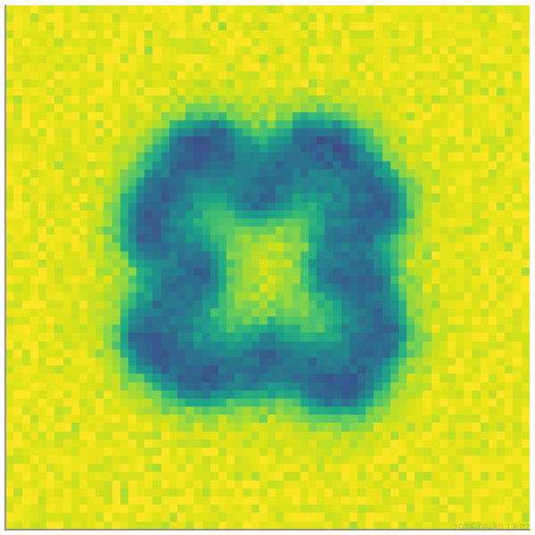
Thumbnail

stamp_output()

[Generated: 2026-06-30 13:02]

🏷 Tags: synthetic, overdamped, SPDE, experimental, reaction-diffusion, 2D, sparsification, multi-experiment