Custom basis with extras — multi-experiment traps

Build a hand-crafted basis with make_basis() that reads experiment-specific metadata from extras.

This is the recommended pattern when your basis functions depend on per-experiment information — trap centres, box sizes, external fields, etc. Each experiment stores its own metadata in extras_global, and the inference engine automatically threads it to the basis at evaluation time.

Here we simulate three 2D experiments with different trap centres and different temperatures. A custom basis encodes displacement from the trap centre (read from extras), and the joint inference recovers the shared spring constant across all conditions.

Tags

synthetic · overdamped · 2D · custom-basis · extras · multi-experiment

Define the true model and simulate

Two experiments share the same force law \(F(x) = -k\,(x - x_0)\) but each has a different trap centre \(x_0\) and a different temperature (diffusion coefficient \(D\)). Both the trap centre and the temperature are stored in extras_global.

from SFI.langevin import OverdampedProcess
from SFI import make_sf

dim = 2
k_true = 2.0
dt = 0.01
Nsteps = 50_000
seed = 42

experiments = [
    {"trap_centre": jnp.array([1.0, 0.5]),  "D": 0.2},
    {"trap_centre": jnp.array([-0.5, 1.0]), "D": 0.5},
    {"trap_centre": jnp.array([0.0, -0.8]), "D": 1.0},
]


def centred_ou_force(x, *, extras):
    """Force toward a trap centre read from extras."""
    x0 = extras["trap_centre"]
    return -k_true * (x - x0)


F_sf = make_sf(centred_ou_force, dim=dim, rank=1, extras_keys=("trap_centre",))

key = random.PRNGKey(seed)
collections = []
for i, exp in enumerate(experiments):
    x0 = exp["trap_centre"]
    D_i = exp["D"]
    proc = OverdampedProcess(F_sf, D=D_i)
    proc.set_extras(extras_global={"trap_centre": x0})
    proc.initialize(x0 + 0.1 * jnp.ones(dim))
    key, sub = random.split(key)
    ds = proc.simulate(dt=dt, Nsteps=Nsteps, key=sub, prerun=200, oversampling=10)
    collections.append(ds)
    print(f"Experiment {i+1}: trap at {np.array(x0)}, D={D_i}, "
          f"{ds.T} frames")

coll = collections[0].concat(collections[1:], weights="pool")

Experiment 1: trap at [1.  0.5], D=0.2, 50000 frames
Experiment 2: trap at [-0.5  1. ], D=0.5, 50000 frames
Experiment 3: trap at [ 0.  -0.8], D=1.0, 50000 frames

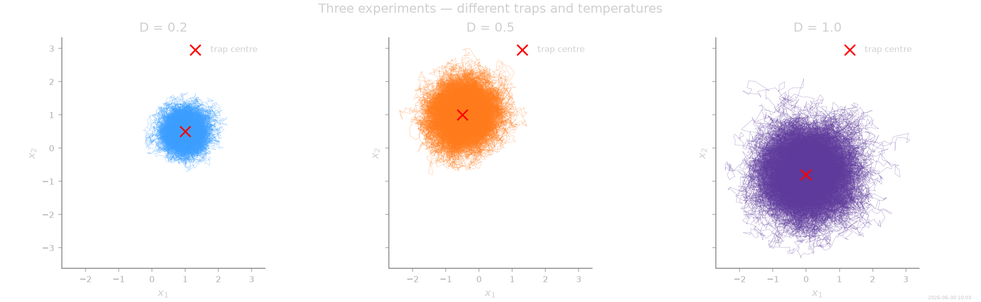
Visualise the experiments

Three experiments with different trap centres and temperatures. Warmer experiments (larger D) show broader fluctuations around the trap.

fig, axes = plt.subplots(1, 3, figsize=(13, 4), sharex=True, sharey=True)
exp_colors = [SFI_COLORS["data"], SFI_COLORS["exact"], SFI_COLORS["bootstrap"]]
for i, (ax, exp, c) in enumerate(zip(axes, experiments, exp_colors)):
    x0 = exp["trap_centre"]
    phase2d(coll, dataset=i, color=c, linewidth=0.3, alpha=0.5, ax=ax)
    ax.scatter(*np.array(x0), marker="x", s=100, color="red", zorder=5,
              label="trap centre")
    ax.set_xlabel("$x_1$")
    ax.set_ylabel("$x_2$")
    ax.set_title(f"D = {exp['D']}")
    ax.legend(fontsize=8)
    ax.set_aspect("equal")
for ax in axes:
    ax.autoscale()
fig.suptitle("Three experiments — different traps and temperatures")
plt.show()

Build a custom basis using make_basis

The key idea is that our basis function reads the trap centre from extras, so the same basis object works for both experiments. The inference engine handles threading the correct extras for each dataset.

We build two families of features:

1. Centred polynomials — monomials of \((x - x_0)\). This is a custom basis that shifts the polynomial origin per experiment.

2. Standard monomials — for comparison, the usual un-centred basis.

from SFI.statefunc import make_basis


def centred_displacement(x, *, extras):
    """Return (x - x0) as a vector basis (rank 1, 1 feature)."""
    x0 = extras["trap_centre"]
    return (x - x0)[:, None]  # shape (dim, 1)


def centred_quadratic(x, *, extras):
    """Return |x - x0|^2 as a scalar basis (rank 0, 1 feature)."""
    x0 = extras["trap_centre"]
    dx = x - x0
    return jnp.sum(dx ** 2, keepdims=True)  # shape (1,)


B_disp = make_basis(centred_displacement, dim=dim, rank=1, n_features=1,
                    extras_keys=("trap_centre",), labels=["x−x₀"])
B_quad = make_basis(centred_quadratic, dim=dim, rank=0, n_features=1,
                    extras_keys=("trap_centre",), labels=["|x−x₀|²"])

# Vectorise the scalar quadratic so it can contribute to each force component
B_custom = B_disp & (B_quad.vectorize(dim))

Infer with the custom basis

from SFI import OverdampedLangevinInference

inf = OverdampedLangevinInference(coll)
inf.compute_diffusion_constant()
inf.infer_force_linear(B_custom, M_mode="Ito")
inf.compute_force_error()

inf.print_report()

  --- StochasticForceInference Report ---
Average diffusion tensor:
 [[ 0.556247   -0.00275321]
 [-0.00275321  0.55038416]]
Measurement noise tensor:
 [[5.5409389e-05 2.2692930e-05]
 [2.2692922e-05 1.0588136e-04]]
Force estimated information: 1574.989990234375
Force: estimated normalized mean squared error (sampling only): 0.0009523870808766688

  Force Coefficient Table
  ───────────────────────────────────────────────────────────────────
  #    Label        Coefficient       Std.Err     SNR  Sig
  ───────────────────────────────────────────────────────────────────
  0    x−x₀        -2.07429e+00   3.69965e-02    56.1  **
  1    |x−x₀|²·e0   5.20996e-02   3.05381e-02     1.7  ·
  2    |x−x₀|²·e1   5.99427e-02   3.03499e-02     2.0  ·
  ───────────────────────────────────────────────────────────────────
  3/3 basis functions in support, sig: 1* / 1** / 0*** (|SNR| ≥ 2 / 10 / 100)
  (Std.err. reflects sampling error only; discretization bias is not included.)

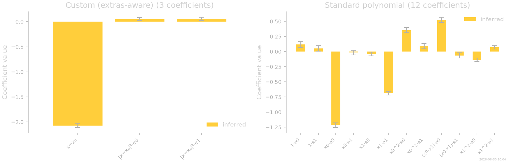
Compare to a standard polynomial basis (un-centred)

Without the extras-aware shift, a polynomial basis needs higher order to capture forces centred at different positions. With three experiments at three temperatures the gap is even larger.

from SFI.bases import monomials_up_to

B_poly = monomials_up_to(order=2, dim=dim, rank='vector')

inf2 = OverdampedLangevinInference(coll)
inf2.compute_diffusion_constant()
inf2.infer_force_linear(B_poly, M_mode="Ito")
inf2.compute_force_error()

from SFI.utils.formatting import print_model_comparison

print(print_model_comparison(
    [inf, inf2],
    ["Custom (extras-aware)", "Standard polynomial"],
    metrics=["n_params", "force_predicted_MSE"],
))

Model Comparison
                Model  n_params  force_predicted_MSE
────────────────────────────────────────────────────
Custom (extras-aware)         3            0.0009524
  Standard polynomial        12             0.008073

Coefficient comparison

The custom basis has just 3 coefficients encoding the physics (displacement from trap) while the polynomial needs 12 to approximate the same force from three shifted traps at different temperatures.

fig, axes = plt.subplots(1, 2, figsize=(11, 3.5))

for ax, inf_i, title in zip(axes, [inf, inf2],
                             ["Custom (extras-aware)", "Standard polynomial"]):
    c = np.asarray(inf_i.force_coefficients)
    plot_recovery_bar(
        inf_i.force_coefficients,
        np.asarray(inf_i.force_support),
        stderr=inf_i.force_coefficients_stderr,
        labels=getattr(inf_i, "force_basis_labels", None),
        ax=ax,
    )
    ax.set_title(f"{title} ({len(c)} coefficients)")

plt.show()

Summary

Pattern	When to use
make_basis(f, extras_keys=(...))	Basis depends on per-experiment metadata (trap centres, box sizes, …)
monomials_up_to(..., rank='vector')	Standard polynomial dictionary — the default starting point
B1 & B2	Concatenate features from different basis families
B.vectorize(dim)	Lift a scalar basis to vector rank for force inference

stamp_output()

[Generated: 2026-06-30 10:04]

🏷 Tags: synthetic, overdamped, 2D, custom-basis, extras, multi-experiment