Note
Go to the end to download the full example code.
Neural-network force field — Müller-Brown potential
Infer the 2D force field of the Müller-Brown potential energy surface with a neural network (multi-layer perceptron), built entirely from SFI’s compositional basis operations, and compare with polynomial-basis inference.
Note
This is an advanced example: it fits a nonlinear-in-θ force
family with the parametric estimator (infer_force()), which runs
frozen-precision L-BFGS for PSF models. Start with the main
gallery if you are new to SFI.
This example demonstrates:
Building an MLP force model by chaining
.rank_to_features(),.dense(),.elementwisemap(), and.features_to_rank()on aBasisobject — a natural dim → H → H → dim architecture.Running
infer_forceon the resulting parametric state function (PSF) — the nonlinear-in-θ L-BFGS path.Head-to-head comparison with polynomial (linear) inference.
Note
The key compositional operations for neural networks are:
.rank_to_features()— folds spatial (rank) axes into the feature axis, turning a vector into a flat feature vector..dense(n, weight=…, bias=…)— learnable affine layer on the feature axis..elementwisemap(jnp.tanh)— activation function..features_to_rank(1)— unfolds features back into spatial axes, turning the output back into a vector field.
These reshape operations are lossless and invertible:
expr.rank_to_features().features_to_rank(expr.rank) is the
identity.
Tags
synthetic · overdamped · nonlinear · neural-network · 2D · Müller-Brown
System: Müller-Brown potential energy surface
The Müller-Brown potential is a classic 2D benchmark from computational chemistry with three local minima connected by two saddle points:
The force is \(\mathbf{F} = -\nabla V\). We rescale by \(\alpha = 0.01\) so that forces are \(\mathcal{O}(1)\).
from SFI.langevin import OverdampedProcess
from SFI.statefunc import make_sf

# Standard Müller-Brown parameters
_A = jnp.array([-200.0, -100.0, -170.0, 15.0])
_a = jnp.array([-1.0, -1.0, -6.5, 0.7])
_b = jnp.array([0.0, 0.0, 11.0, 0.6])
_c = jnp.array([-10.0, -10.0, -6.5, 0.7])
_xbar = jnp.array([1.0, 0.0, -0.5, -1.0])
_ybar = jnp.array([0.0, 0.5, 1.5, 1.0])

ALPHA = 0.01  # rescaling factor


def muller_brown_potential(xy):
    """Müller-Brown potential (rescaled)."""
    x, y = xy[0], xy[1]
    exponents = (
        _a * (x - _xbar) ** 2
        + _b * (x - _xbar) * (y - _ybar)
        + _c * (y - _ybar) ** 2
    )
    return ALPHA * jnp.sum(_A * jnp.exp(exponents))


_neg_grad_V = jax.grad(lambda xy: -muller_brown_potential(xy))


def mb_force(x):
    """Force F = −∇V for the rescaled Müller-Brown potential."""
    return _neg_grad_V(x)


# Simulation parameters
D0 = 0.5
dt = 0.01
Nsteps = 15_000
seed = 42

F_exact = make_sf(mb_force, dim=2, rank=1)
proc = OverdampedProcess(F_exact, D=D0 * jnp.eye(2))
proc.initialize(jnp.array([-0.5, 1.5]))

key = random.PRNGKey(seed)
coll = proc.simulate(dt=dt, Nsteps=Nsteps, key=key, prerun=500, oversampling=10)
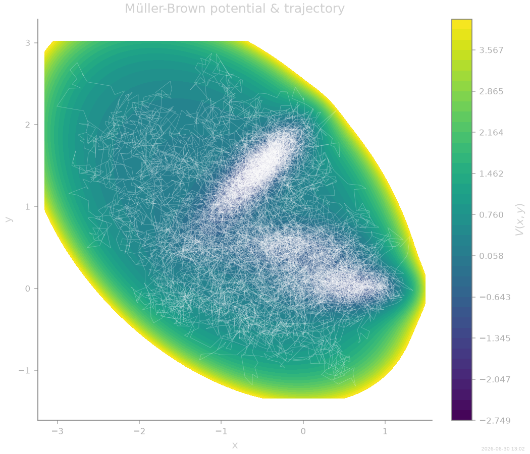
Potential landscape and trajectory
The contour plot shows the three-well structure. Thermal noise (\(D = 0.5\)) allows the particle to explore all basins.
_, X_full, _ = coll.to_arrays(dataset=0)   # (T,), (T, N, d), (T, N)
X_traj = np.asarray(X_full[:, 0, :])       # single particle -> (T, 2)

# Bounding box from trajectory (with margin) — used throughout
pad = 0.15
xlo, xhi = float(X_traj[:, 0].min()) - pad, float(X_traj[:, 0].max()) + pad
ylo, yhi = float(X_traj[:, 1].min()) - pad, float(X_traj[:, 1].max()) + pad

# Evaluation grid for potential
xg = np.linspace(xlo, xhi, 120)
yg = np.linspace(ylo, yhi, 120)
XG, YG = np.meshgrid(xg, yg)
pts_grid = jnp.stack([XG.ravel(), YG.ravel()], axis=-1)
V_grid = np.asarray(jax.vmap(muller_brown_potential)(pts_grid)).reshape(XG.shape)

# Data-consistent scales: evaluate along trajectory to set contour/quiver ranges
_X_sub = jnp.array(X_traj[::10])
V_data = np.asarray(jax.vmap(muller_brown_potential)(_X_sub))
F_data_mag = np.linalg.norm(np.asarray(F_exact(_X_sub)), axis=-1)
F_clip = float(np.percentile(F_data_mag, 99)) * 2  # ceiling for quiver arrows
V_lo, V_hi = float(V_data.min()), float(V_data.max())
V_margin = 0.3 * (V_hi - V_lo)
levels = np.linspace(V_lo - V_margin, V_hi + V_margin, 40)

fig, ax = plt.subplots(figsize=(7, 6))
cs = ax.contourf(XG, YG, V_grid, levels=levels, cmap="viridis")
phase2d(coll, dims=(0, 1), color="white", alpha=0.3, linewidth=0.4, ax=ax)
ax.set_title("Müller-Brown potential & trajectory")
plt.colorbar(cs, ax=ax, label=r"$V(x, y)$")
plt.show()
Polynomial (linear) inference — baseline
Monomials up to degree 5 give 21 scalar and 42 vectorised features. This is a standard SFI workflow: the polynomial captures smooth, low-order trends but cannot represent the sharp Gaussian channels of the Müller-Brown surface.
from SFI import OverdampedLangevinInference
from SFI.bases import monomials_up_to

poly_order = 5
B_poly = monomials_up_to(order=poly_order, dim=2, rank='vector')

inf = OverdampedLangevinInference(coll)
inf.compute_diffusion_constant()

inf.infer_force_linear(B_poly, M_mode="Ito")
inf.compare_to_exact(model_exact=proc, maxpoints=5000)
nmse_poly = float(inf.NMSE_force)
force_poly = inf.force_inferred
theta_poly = jnp.asarray(inf.force_coefficients_full)

inf.print_report()
  --- StochasticForceInference Report ---
Average diffusion tensor:
 [[0.45851895 0.00678546]
 [0.00678546 0.46321774]]
Measurement noise tensor:
 [[ 3.5211002e-04 -4.9641501e-05]
 [-4.9641509e-05  2.2957200e-04]]
Normalized MSE (force):     1.1934
Normalized MSE (diffusion): 0.0075

  Force Coefficient Table
  ───────────────────────────────────────────────
  #    Label            Coefficient  Sig
  ───────────────────────────────────────────────
  0    1·e0             8.48264e-01  ·
  1    1·e1             7.91052e-01  ·
  2    x0·e0            3.94022e-01  ·
  3    x0·e1           -3.60741e-01  ·
  4    x1·e0           -2.25566e+00  ·
  5    x1·e1           -3.12494e+00  ·
  6    x0^2·e0         -1.42961e+00  ·
  7    x0^2·e1         -2.34853e-01  ·
  8    (x0·x1)·e0      -2.81542e+00  ·
  9    (x0·x1)·e1      -6.78079e+00  ·
  10   x1^2·e0         -2.61970e+00  ·
  11   x1^2·e1          7.70487e-01  ·
  12   x0^3·e0         -2.24618e+00  ·
  13   x0^3·e1          1.04770e+00  ·
  14   (x0^2·x1)·e0     3.01798e+00  ·
  15   (x0^2·x1)·e1    -5.41184e+00  ·
  16   (x0·x1^2)·e0    -2.59711e+00  ·
  17   (x0·x1^2)·e1     3.14690e+00  ·
  18   x1^3·e0          1.44717e+00  ·
  19   x1^3·e1          3.53814e+00  ·
  20   x0^4·e0         -8.91240e-01  ·
  21   x0^4·e1          1.48724e-02  ·
  22   (x0^3·x1)·e0     4.24694e+00  ·
  23   (x0^3·x1)·e1    -1.60837e+00  ·
  24   (x0^2·x1^2)·e0  -6.31833e-03  ·
  25   (x0^2·x1^2)·e1   6.38271e+00  ·
  26   (x0·x1^3)·e0     3.12109e+00  ·
  27   (x0·x1^3)·e1     4.81721e+00  ·
  28   x1^4·e0          1.08342e+00  ·
  29   x1^4·e1         -1.99358e+00  ·
  30   x0^5·e0         -1.39567e-01  ·
  31   x0^5·e1         -2.67660e-01  ·
  32   (x0^4·x1)·e0     9.72966e-01  ·
  33   (x0^4·x1)·e1    -9.75972e-01  ·
  34   (x0^3·x1^2)·e0  -2.74626e-01  ·
  35   (x0^3·x1^2)·e1  -6.44915e-01  ·
  36   (x0^2·x1^3)·e0  -4.37884e-01  ·
  37   (x0^2·x1^3)·e1  -2.33460e+00  ·
  38   (x0·x1^4)·e0    -1.14739e+00  ·
  39   (x0·x1^4)·e1    -2.39564e+00  ·
  40   x1^5·e0         -5.65339e-01  ·
  41   x1^5·e1          1.00656e-01  ·
  ───────────────────────────────────────────────
  42/42 basis functions in support
Neural-network architecture (MLP)
We build a two-hidden-layer MLP entirely within SFI’s expression tree:
Start from position —
X(dim=2)is a rank-1 basis with 1 feature, representing the position vector \(\mathbf{x} \in \mathbb{R}^2\).Flatten to features —
.rank_to_features()folds the spatial axis into features, giving a rank-0 expression withdimfeatures. Now \((x, y)\) lives on the feature axis where dense layers operate.Hidden layers —
dense(32) → tanh → dense(32) → tanh.Output —
dense(dim)producesdimfeatures, and.features_to_rank(1)reinterprets them as a rank-1 vector field with 1 feature — exactly the PSF shapeinfer_force()expects.
This gives a natural 2 → 64 → 64 → 64 → 2 MLP for the force field.
from SFI.bases import X

dim = 2
H = 32  # hidden layer width

mlp = (
    X(dim=dim)                                            # rank-1, 1 feature
    .rank_to_features()                                   # rank-0, dim features
    .dense(H, weight="W1", bias="b1")                    # rank-0, H features
    .elementwisemap(jnp.tanh)                             # activation
    .dense(H, weight="W2", bias="b2")                    # rank-0, H features
    .elementwisemap(jnp.tanh)                             # activation
    .dense(dim, weight="W3", bias="b3")                  # rank-0, dim features
    .features_to_rank(1)                                  # rank-1, 1 feature
)

n_params = mlp.template.size
print(f"MLP architecture: {dim} → {H} → {H} → {dim}   ({n_params} parameters)")
MLP architecture: 2 → 32 → 32 → 2 (1218 parameters)
Parameter initialisation
Xavier/Glorot initialisation breaks weight symmetry and prevents dead neurons at start-up. Biases are set to zero.
theta0 = {}
init_key = random.PRNGKey(123)

for name, shape in [
    ("W1", (dim, H)),  ("b1", (H,)),
    ("W2", (H, H)),   ("b2", (H,)),
    ("W3", (H, dim)), ("b3", (dim,)),
]:
    init_key, subkey = random.split(init_key)
    if name.startswith("W"):
        fan_in, fan_out = shape
        std = jnp.sqrt(2.0 / (fan_in + fan_out))
        theta0[name] = std * random.normal(subkey, shape)
    else:
        theta0[name] = jnp.zeros(shape)
NN force inference (nonlinear optimisation)
For a (nonlinear-in-θ) PSF the parametric infer_force() minimises
the windowed-precision NLL of the single-step flow residuals with
frozen-precision L-BFGS, re-profiling (D, Λ) once at the fitted
parameters. We raise the inner L-BFGS budget for the NN landscape.
A fresh inference object keeps the NN fit cleanly separated from the
linear baseline.
# The inner L-BFGS budget is deliberately *shallow*: deep inner solves
# against the provisional frozen precision overfit the wrong metric
# before the (D, Λ) reprofile can correct it (the classic IRLS trap;
# quantified in the companion NN study).
inf_nn = OverdampedLangevinInference(coll)
inf_nn.infer_force(
    mlp, theta0,
    inner_maxiter=60,
    max_outer=2,
)

inf_nn.compare_to_exact(model_exact=proc, maxpoints=5000)
nmse_nn = float(inf_nn.NMSE_force)

nn_info = inf_nn.metadata["force_parametric_info"]
inf_nn.print_report()
print(f"L-BFGS IRLS: {nn_info['outer_iterations']} outer steps, "
      f"best loss = {nn_info['loss']:.6g}")
  --- StochasticForceInference Report ---
Average diffusion tensor:
 [[0.4787258  0.00323607]
 [0.00323607 0.47907156]]
Measurement noise tensor:
 [[ 2.0642059e-04 -2.2953236e-05]
 [-2.2953236e-05  1.4214119e-04]]
Normalized MSE (force):     0.9623
Normalized MSE (diffusion): 0.0020

  Force Coefficient Table
  ───────────────────────────────────────
  #     Label   Coefficient  Sig
  ───────────────────────────────────────
  0     b0      5.00876e-01  ·
  1     b1      1.19373e+00  ·
  2     b2      8.12275e-01  ·
  3     b3      7.16416e-01  ·
  4     b4      4.60556e-01  ·
  5     b5      1.22094e+00  ·
  6     b6      4.17268e-01  ·
  7     b7      1.26507e+00  ·
  8     b8      6.62400e-01  ·
  9     b9     -1.67042e+00  ·
  10    b10     6.00304e-01  ·
  11    b11     4.35963e-01  ·
  12    b12     2.07249e+00  ·
  13    b13    -9.05615e-01  ·
  14    b14     4.83769e-01  ·
  15    b15    -6.96149e-01  ·
  16    b16     2.85093e+00  ·
  17    b17     5.35233e-01  ·
  18    b18     6.35904e-03  ·
  19    b19    -2.78124e-01  ·
  20    b20    -9.83541e-01  ·
  21    b21    -5.73202e-01  ·
  22    b22    -1.35522e+00  ·
  23    b23    -4.29106e-02  ·
  24    b24     1.83330e-01  ·
  25    b25    -4.68333e-01  ·
  26    b26    -6.25253e-01  ·
  27    b27    -6.01221e-01  ·
  28    b28    -6.11208e-01  ·
                    ...
  1189  b1189   1.83314e+00  ·
  1190  b1190  -1.74249e-01  ·
  1191  b1191   8.82200e-02  ·
  1192  b1192   5.70192e-01  ·
  1193  b1193  -5.92606e-01  ·
  1194  b1194   1.87948e-01  ·
  1195  b1195   6.30179e-01  ·
  1196  b1196   3.06235e-01  ·
  1197  b1197  -9.65222e-01  ·
  1198  b1198  -3.05273e-01  ·
  1199  b1199   6.91785e-01  ·
  1200  b1200   4.22403e-01  ·
  1201  b1201   5.02646e-02  ·
  1202  b1202  -9.97526e-01  ·
  1203  b1203   1.57719e+00  ·
  1204  b1204   4.70988e-01  ·
  1205  b1205  -6.26268e-01  ·
  1206  b1206   1.24521e-01  ·
  1207  b1207  -4.20746e-01  ·
  1208  b1208   4.22089e-01  ·
  1209  b1209  -1.06282e+00  ·
  1210  b1210  -3.50972e-01  ·
  1211  b1211   1.12680e+00  ·
  1212  b1212   1.05579e-01  ·
  1213  b1213  -3.37470e-01  ·
  1214  b1214  -4.02635e-01  ·
  1215  b1215   1.10278e+00  ·
  1216  b1216  -2.06156e+00  ·
  1217  b1217   3.19577e-01  ·
  ───────────────────────────────────────
  1218/1218 basis functions in support
L-BFGS IRLS: 2 outer steps, best loss = 14760.6
Last-layer Gauss–Newton polish
The recommended finishing move: freeze the warm-started network
body and refit the final dense layer as a linear basis through
the fast Gauss–Newton path. The hidden activations become feature
functions z_h(x)·e_i, so the last layer’s weights are ordinary
linear coefficients — solved in seconds, with proper error bars.
from SFI.statefunc import make_basis

theta_nn = mlp.unflatten_params(inf_nn.force_coefficients_full)


def body_features(x, *, mask=None, extras=None):
    z = jnp.tanh(theta_nn["W1"].T @ x + theta_nn["b1"])
    z = jnp.tanh(theta_nn["W2"].T @ z + theta_nn["b2"])
    feats = jnp.einsum("h,ij->ihj", z, jnp.eye(dim)).reshape(dim, H * dim)
    return jnp.concatenate([feats, jnp.eye(dim)], axis=1)   # + bias features


B_last = make_basis(body_features, dim=dim, rank=1, n_features=H * dim + dim)

inf_polish = OverdampedLangevinInference(coll)
inf_polish.infer_force(B_last, eiv=False)   # clean data: symmetric GN
inf_polish.compare_to_exact(model_exact=proc, maxpoints=5000)
nmse_polish = float(inf_polish.NMSE_force)
force_nn = inf_polish.force_inferred        # use the polished field below
inf_polish.print_report()
nmse_nn = min(nmse_nn, nmse_polish)
  --- StochasticForceInference Report ---
Average diffusion tensor:
 [[5.0081021e-01 1.2456917e-04]
 [1.2456917e-04 4.9610811e-01]]
Measurement noise tensor:
 [[0. 0.]
 [0. 0.]]
Normalized MSE (force):     0.4461
Normalized MSE (diffusion): 0.0000

  Force Coefficient Table
  ──────────────────────────────────────
  #    Label   Coefficient  Sig
  ──────────────────────────────────────
  0    b0      1.98640e+01  ·
  1    b1     -1.78866e+00  ·
  2    b2     -1.52721e+00  ·
  3    b3      3.62016e-01  ·
  4    b4      2.84040e-01  ·
  5    b5      1.56833e+01  ·
  6    b6     -1.59602e+00  ·
  7    b7     -4.97924e+00  ·
  8    b8      3.57613e+00  ·
  9    b9      4.99987e+00  ·
  10   b10    -9.24296e+00  ·
  11   b11     5.58453e+00  ·
  12   b12     5.91288e+00  ·
  13   b13    -5.29000e+00  ·
  14   b14     2.51587e+01  ·
  15   b15    -2.40111e+01  ·
  16   b16    -8.78174e-01  ·
  17   b17    -2.72912e+00  ·
  18   b18     7.53283e+00  ·
  19   b19     9.08562e+00  ·
  20   b20    -1.51117e+01  ·
  21   b21     1.38515e+01  ·
  22   b22    -9.23787e-01  ·
  23   b23    -1.33868e+00  ·
  24   b24     6.20386e+00  ·
  25   b25     3.89341e+00  ·
  26   b26     4.32029e+00  ·
  27   b27     4.34533e+00  ·
  28   b28     1.34940e+01  ·
                   ...
  37   b37     2.72551e+00  ·
  38   b38    -1.35872e+00  ·
  39   b39     1.31051e+01  ·
  40   b40    -1.28446e+00  ·
  41   b41    -9.70066e-01  ·
  42   b42     1.78234e+01  ·
  43   b43    -1.24772e+01  ·
  44   b44     3.22466e-01  ·
  45   b45    -1.87286e+00  ·
  46   b46     7.99941e-01  ·
  47   b47     2.38823e+00  ·
  48   b48    -2.58208e+01  ·
  49   b49     6.41823e-01  ·
  50   b50    -1.58897e+00  ·
  51   b51     9.68980e-01  ·
  52   b52     4.49965e-02  ·
  53   b53    -1.12632e+00  ·
  54   b54     7.06719e+00  ·
  55   b55    -8.19713e+00  ·
  56   b56     5.01393e-01  ·
  57   b57    -1.47743e+01  ·
  58   b58     7.17478e-01  ·
  59   b59     2.87564e+00  ·
  60   b60    -1.95322e+01  ·
  61   b61     1.32176e+01  ·
  62   b62    -1.65022e+00  ·
  63   b63     7.29620e+00  ·
  64   b64    -1.54229e+01  ·
  65   b65     4.49104e+00  ·
  ──────────────────────────────────────
  66/66 basis functions in support
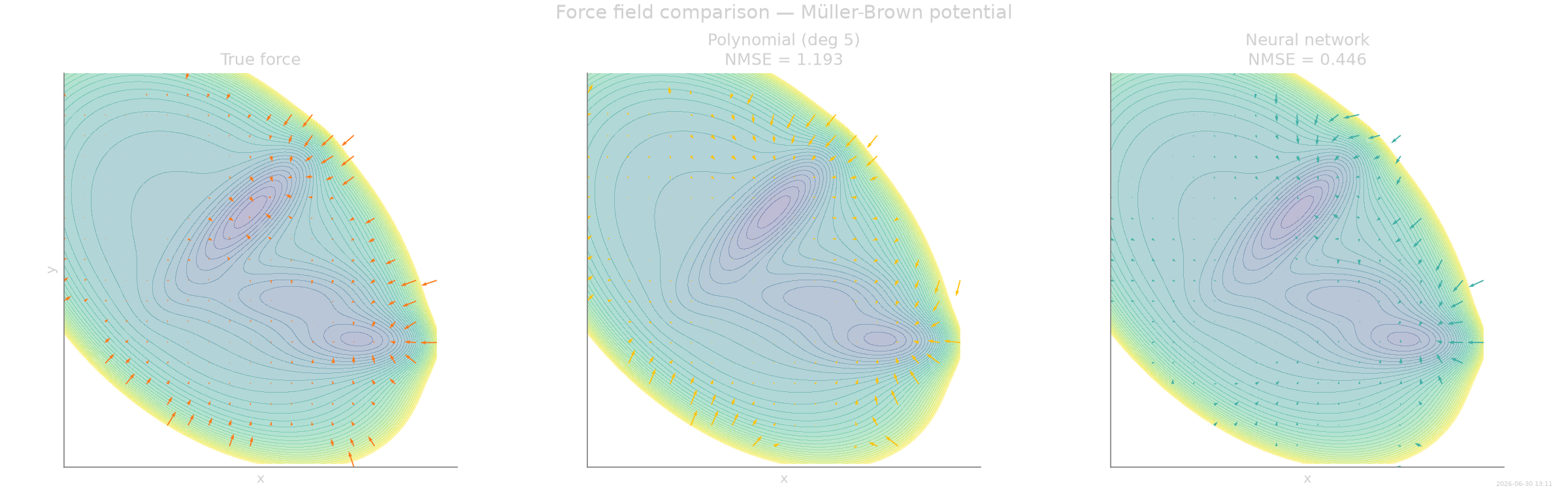
Force field comparison
Quiver plots of the true, polynomial, and NN force fields on a regular 2D grid clipped to the region explored by the trajectory. The neural network closely tracks the true force in the narrow saddle regions where the polynomial deteriorates.
# Quiver grid: ``plot_field`` drops arrows in unvisited cells
# (``mask_unvisited``) and caps each arrow at ``F_clip`` (``clip_magnitude``),
# so all three panels share one arrow scale.
Nq = 20
_rad = 0.5 * float((X_traj.max(axis=0) - X_traj.min(axis=0)).max())
arrow_scale = 1.6 * _rad / (Nq - 1)   # longest arrow ≈ one grid cell

fig, axes = plt.subplots(1, 3, figsize=(16, 5), sharex=True, sharey=True)

titles = [
    "True force",
    f"Polynomial (deg {poly_order})\nNMSE = {nmse_poly:.3f}",
    f"Neural network\nNMSE = {nmse_nn:.3f}",
]
fields = [F_exact, force_poly, force_nn]
colors = [SFI_COLORS["exact"], SFI_COLORS["inferred"], SFI_COLORS["highlight"]]

for ax, title, field, color in zip(axes, titles, fields, colors):
    ax.contourf(XG, YG, V_grid, levels=levels, cmap="viridis", alpha=0.35)
    plt.sca(ax)
    plot_field(
        coll, field, N=Nq, color=color,
        mask_unvisited=True, clip_magnitude=F_clip,
        autoscale=True, scale=arrow_scale,
    )
    ax.set_title(title)
    ax.set_xlabel("x")

axes[0].set_ylabel("y")
fig.suptitle("Force field comparison — Müller-Brown potential", fontsize=14)
plt.show()
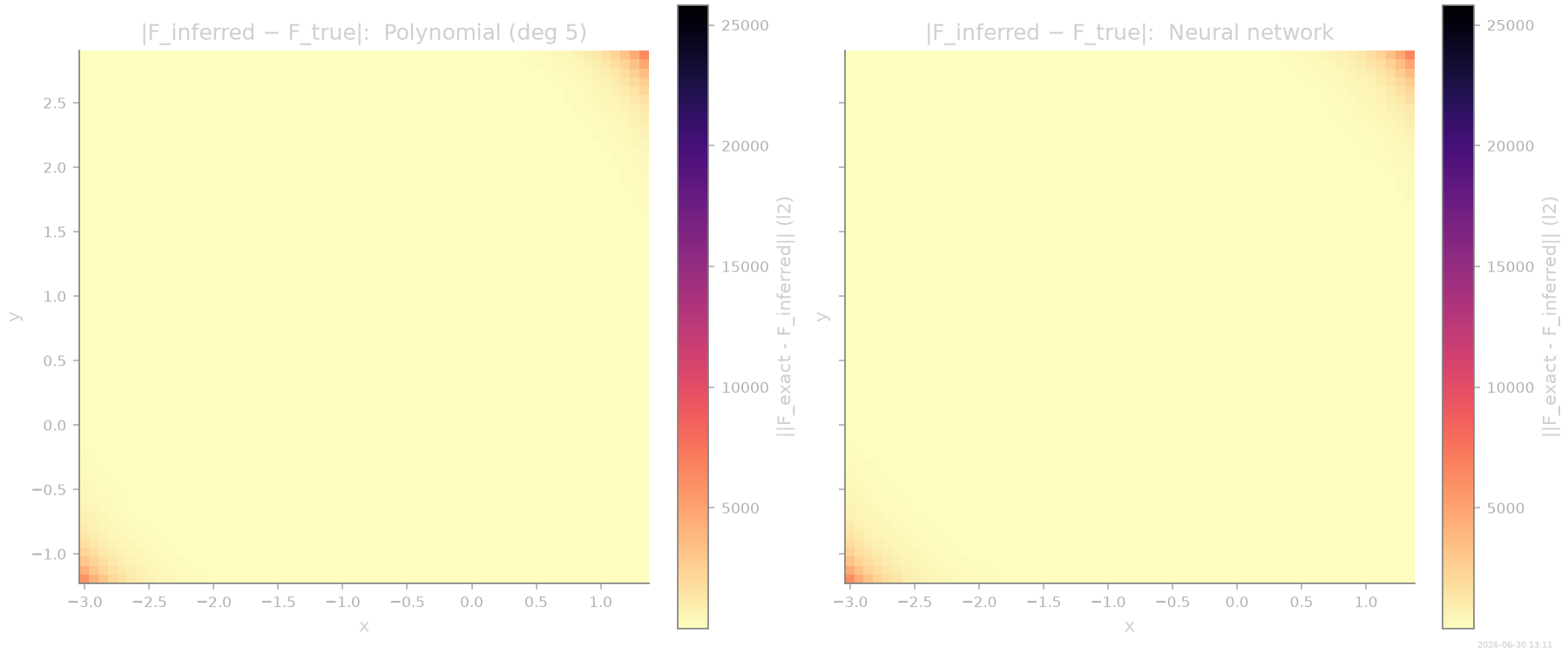
Point-wise force error
The error map highlights where each model fails. The polynomial concentrates error near saddle points and channel walls; the NN distributes residual error more uniformly and at a lower level.
# Shared colour ceiling so the two error maps are directly comparable.
_egx, _egy = np.meshgrid(np.linspace(xlo, xhi, 60), np.linspace(ylo, yhi, 60))
_epts = jnp.stack([_egx.ravel(), _egy.ravel()], axis=-1)
_Fe = np.asarray(F_exact(_epts))
err_vmax = float(max(
    np.linalg.norm(np.asarray(force_poly(_epts)) - _Fe, axis=-1).max(),
    np.linalg.norm(np.asarray(force_nn(_epts)) - _Fe, axis=-1).max(),
))

fig, axes = plt.subplots(1, 2, figsize=(12, 5), sharex=True, sharey=True)
plot_field_error(coll, force_poly, F_exact, ax=axes[0], cmap="magma_r", vmax=err_vmax)
axes[0].set_title(f"|F_inferred − F_true|:  Polynomial (deg {poly_order})")
plot_field_error(coll, force_nn, F_exact, ax=axes[1], cmap="magma_r", vmax=err_vmax)
axes[1].set_title("|F_inferred − F_true|:  Neural network")
plt.show()
Summary
The MLP force field captures the non-polynomial Gaussian landscape of the Müller-Brown surface more faithfully than a degree-5 monomial basis. Parametric SFI refines the polynomial estimate using RK4 splitting and Gauss–Newton, improving accuracy without switching to a neural-network architecture.
import time as _time

F_psf_poly = B_poly.to_psf()
theta0_parametric = {"coeff": theta_poly}

inf_parametric = OverdampedLangevinInference(coll)
t0_parametric = _time.perf_counter()
inf_parametric.infer_force(F_psf_poly, theta0_parametric)
t_parametric = _time.perf_counter() - t0_parametric
inf_parametric.compare_to_exact(model_exact=proc, maxpoints=5000)

print()
print(print_model_comparison(
    [inf, inf_parametric, inf_polish],
    ["Poly (deg 5)", "Poly + Parametric SFI", "NN (MLP)"],
    metrics=["n_params", "NMSE_force"],
    extra_cols={"Time (s)": {"Poly + Parametric SFI": round(t_parametric, 1)}},
))
Model Comparison
                Model  n_params  NMSE_force  Time (s)
─────────────────────────────────────────────────────
         Poly (deg 5)        42       1.193         —
Poly + Parametric SFI        42       1.373      67.1
             NN (MLP)        66      0.4461         —
Thumbnail
stamp_output()
[Generated: 2026-06-30 13:13]
Total running time of the script: (10 minutes 47.538 seconds)