Lotka–Volterra ecosystem — sparse network recovery

Recover the sparse interaction network of a 6-species Lotka–Volterra ecosystem from a heavily downsampled stochastic trajectory, using a custom polynomial-of-exponential basis and PASTIS model selection.

The model lives in log-population coordinates \(x_i = \log n_i\), where the force takes the simple form

\[F_i(x) = r_i + \sum_j A_{ij}\,e^{x_j}\]

with growth rates \(r\) and a sparse interaction matrix \(A\). Only 18 of the 42 candidate parameters are nonzero — PASTIS recovers this structure from downsampled, noisy data.

Note

This example uses SFI’s parametric force estimator (infer_force()). It is needed here: the measurement noise acts through the exponential basis (an errors-in-variables effect) and, together with the stiff nonlinear dynamics, defeats the linear Itô estimator (which does not recover the network). The parametric estimator profiles the noise level and uses the noise-clean skip instrument, and so stays unbiased.

Tags

synthetic · overdamped · nonlinear · sparsity · ecology · custom-basis

System definition

A 6-species Lotka–Volterra ecosystem in log-population coordinates. The interaction matrix \(A\) is deliberately sparse: most pairs of species do not interact. Self-interactions (diagonal) are all negative (density-dependent mortality), while a handful of off-diagonal entries encode predation (+/−) or competition (−/−).

from SFI.langevin import OverdampedProcess
from SFI import make_sf

dim = 6

# Intrinsic growth rates
r = jnp.array([0.50, 0.65, 0.55, 0.65, 0.58, 0.62])

# Interaction matrix (sparse: 18 nonzero entries out of 42 parameters)
A = jnp.array([
    [-0.90, -0.60,  0.00,  0.00,  0.00,  0.00],
    [ 0.00, -0.70, -0.60,  0.00,  0.00,  0.00],
    [+0.60,  0.00, -0.90,  0.00,  0.00, -0.40],
    [ 0.00,  0.00,  0.00, -0.90, -0.50,  0.00],
    [ 0.00,  0.00,  0.00,  0.00, -0.40, -0.60],
    [ 0.00,  0.00, -0.40, +0.40,  0.00, -1.00],
])

D0 = 0.002  # small isotropic noise

dt = 0.01
Nsteps = 40_000
oversampling = 20
seed = 0


def lv_force(x):
    """Lotka–Volterra force in log-population coordinates."""
    return A @ jnp.exp(x) + r


key = random.PRNGKey(seed)
F_sf = make_sf(lv_force, dim=dim, rank=1)

proc = OverdampedProcess(F_sf, D=jnp.eye(dim) * D0)
proc.initialize(jnp.full(dim, -6.0))

key, sub = random.split(key)
coll_clean = proc.simulate(
    dt=dt, Nsteps=Nsteps, key=sub, prerun=0, oversampling=oversampling,
)
print(f"Clean trajectory: {coll_clean.T} frames, dim={coll_clean.d}, dt={dt}")

Clean trajectory: 40000 frames, dim=6, dt=0.01

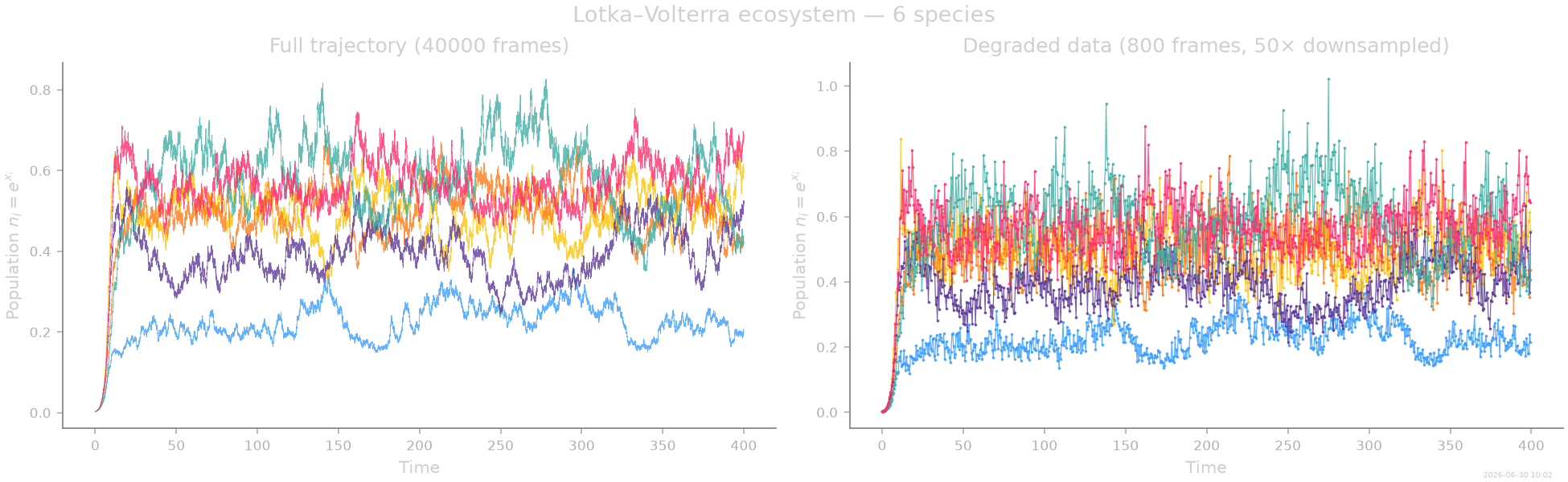
Degrade the data

Downsample the trajectory and add measurement noise to simulate a realistic low-data regime. The inference will use only ~2 000 frames instead of 40 000.

downsample_factor = 50
noise_level = 0.1  # measurement noise in log-population coordinates
coll_degraded = coll_clean.degrade(downsample=downsample_factor, noise=noise_level, seed=42)
print(f"Degraded trajectory: {coll_degraded.T} frames "
      f"(downsampled {downsample_factor}×, effective dt={dt * downsample_factor}, "
      f"noise={noise_level})")

Degraded trajectory: 800 frames (downsampled 50×, effective dt=0.5, noise=0.1)

Population dynamics

Left: the full simulated trajectory (40 000 frames) showing rich oscillatory dynamics of six coexisting species. Right: the downsampled, noisy data actually used for inference.

# Population-space views (n_i = e^{x_i}) for plotting, via the
# ``transform`` hook on ``timeseries`` (exponentiates the log-population
# states on the fly).

Custom polynomial-of-exponential basis

In log-population coordinates the force is linear in the populations \(e^{x_j}\), so the natural basis dictionary is

\[\{1,\; e^{x_1},\; \dots,\; e^{x_6}\}\]

giving 7 scalar features. Vectorising to 6 species yields \(7 \times 6 = 42\) force parameters. The true model uses only 18 of them (6 growth rates + 12 nonzero interactions).

from SFI.statefunc import make_basis

import SFI


def polyexp_basis_func(x):
    """Scalar basis: {1, exp(x_1), ..., exp(x_d)}."""
    return jnp.concatenate([jnp.ones(1), jnp.exp(x)])  # shape (dim+1,)


# Labels: constant + each exponential
basis_labels = ["1"] + [f"exp(x{i+1})" for i in range(dim)]

B_scalar = make_basis(
    polyexp_basis_func, dim=dim, rank=0,
    n_features=dim + 1, labels=basis_labels,
)
B = B_scalar.vectorize(dim)

Inference and sparsification

We fit the force with the parametric estimator (infer_force()), which profiles the measurement-noise level and so stays unbiased on the noisy exponential basis. PASTIS then selects the sparse interaction network from the candidate basis.

# This system sits deep in the noise-dominated regime
# (β = σ²/(2DΔt) ≈ 12): the residual correlations decay slowly, so we
# widen the precision window beyond its default (``extra_radius=3``) —
# the documented escape hatch for β ≫ 1.  The skip-trick instrument
# (on by default) is what removes the errors-in-variables bias here.
inf = SFI.OverdampedLangevinInference(coll_degraded)
inf.infer_force(B, extra_radius=3)
inf.compute_force_error()

inf.sparsify_force(criterion="PASTIS", p=0.1)
inf.compute_force_error()
inf.compare_to_exact(model_exact=proc, maxpoints=2000)

k_sel, support_sel, _, coeffs_sel = inf.force_sparsity_result.select_by_ic("PASTIS")

inf.print_report()

  --- StochasticForceInference Report ---
Average diffusion tensor:
 [[ 0.00556921  0.00182363  0.00438365  0.00395803  0.00392299 -0.00147579]
 [ 0.00182363  0.00449589  0.00046078  0.00119376  0.00223874  0.00026247]
 [ 0.00438365  0.00046078  0.00392082  0.00319596  0.00332776 -0.00205281]
 [ 0.00395803  0.00119376  0.00319596  0.00282903  0.00287611 -0.00124077]
 [ 0.00392299  0.00223874  0.00332776  0.00287611  0.00413586 -0.00227219]
 [-0.00147579  0.00026247 -0.00205281 -0.00124077 -0.00227219  0.00276641]]
Measurement noise tensor:
 [[ 8.0501279e-03 -2.9285561e-04 -2.9264949e-03 -3.1585831e-03
  -3.0075232e-03 -2.0367015e-06]
 [-2.9285561e-04  8.0877161e-03  5.5461889e-04 -8.8109495e-04
  -1.2566745e-03  2.7723200e-04]
 [-2.9264949e-03  5.5461889e-04  1.0033747e-02 -1.8858720e-03
  -2.5273946e-03  2.1461614e-03]
 [-3.1585831e-03 -8.8109495e-04 -1.8858720e-03  9.9254912e-03
  -1.6873083e-03 -9.1600989e-05]
 [-3.0075232e-03 -1.2566745e-03 -2.5273946e-03 -1.6873083e-03
   8.4654232e-03  1.1892261e-03]
 [-2.0367015e-06  2.7723200e-04  2.1461614e-03 -9.1600989e-05
   1.1892261e-03  9.3112867e-03]]
Force estimated information: 390.9839782714844
Force: estimated normalized mean squared error (sampling only): 0.02301883140517039
Normalized MSE (force):     0.0525
Normalized MSE (diffusion): 20752715743232.0000

  Force Coefficient Table
  ───────────────────────────────────────────────────────────────────
  #    Label        Coefficient       Std.Err     SNR  Sig
  ───────────────────────────────────────────────────────────────────
  0    1·e0         5.40734e-01   4.89413e-02    11.0  **
  1    1·e1         6.58438e-01   5.06504e-02    13.0  **
  2    1·e2         5.64812e-01   4.43631e-02    12.7  **
  3    1·e3         6.06781e-01   3.81104e-02    15.9  **
  4    1·e4         5.18866e-01   4.31965e-02    12.0  **
  5    1·e5         6.01181e-01   4.40407e-02    13.7  **
  6    exp(x1)·e0  -1.04409e+00   1.33825e-01     7.8  *
  12   exp(x2)·e0  -6.21589e-01   8.44193e-02     7.4  *
  13   exp(x2)·e1  -7.29395e-01   9.31834e-02     7.8  *
  14   exp(x2)·e2  -3.82674e-01   7.76569e-02     4.9  *
  19   exp(x3)·e1  -5.96242e-01   8.59709e-02     6.9  *
  20   exp(x3)·e2  -7.49845e-01   7.11997e-02    10.5  **
  23   exp(x3)·e5  -4.09869e-01   9.96832e-02     4.1  *
  27   exp(x4)·e3  -7.96447e-01   6.68330e-02    11.9  **
  28   exp(x4)·e4  -5.54260e-01   7.94202e-02     7.0  *
  33   exp(x5)·e3  -5.05734e-01   4.07822e-02    12.4  **
  34   exp(x5)·e4  -5.14312e-01   4.82189e-02    10.7  **
  41   exp(x6)·e5  -6.95784e-01   9.65358e-02     7.2  *
  ───────────────────────────────────────────────────────────────────
  18/42 basis functions in support, sig: 18* / 10** / 0*** (|SNR| ≥ 2 / 10 / 100)
  (Std.err. reflects sampling error only; discretization bias is not included.)
  Zeroed (24): exp(x1)·e1, exp(x1)·e2, exp(x1)·e3, exp(x1)·e4, exp(x1)·e5, exp(x2)·e3, exp(x2)·e4, exp(x2)·e5, exp(x3)·e0, exp(x3)·e3, exp(x3)·e4, exp(x4)·e0, exp(x4)·e1, exp(x4)·e2, exp(x4)·e5, exp(x5)·e0, exp(x5)·e1, exp(x5)·e2, exp(x5)·e5, exp(x6)·e0, exp(x6)·e1, exp(x6)·e2, exp(x6)·e3, exp(x6)·e4

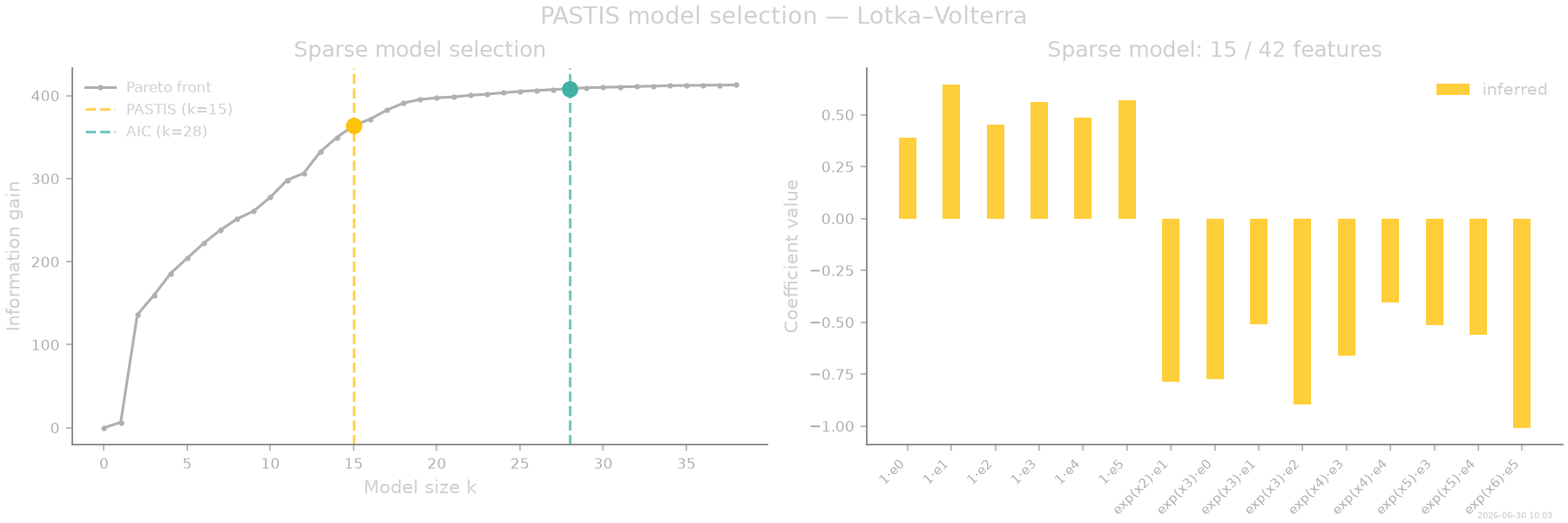
Pareto front and sparse model

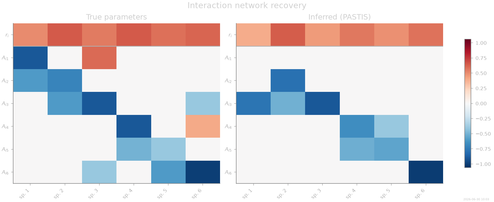
Interaction matrix recovery

The standout result: the inferred sparse coefficients reshaped as a \((d{+}1) \\times d\) parameter matrix (growth rates on top, interaction columns below) compared to the ground truth. Zeros in the true matrix should appear as zeros in the inferred one.

# True parameter matrix: first row = r, rows 1..d = A^T
true_params = np.array(jnp.vstack((r[None, :], A.T)))

# Reconstruct inferred parameter matrix from sparse coefficients
inferred_flat = np.zeros(B.n_features)
inferred_flat[np.array(support_sel)] = np.array(coeffs_sel)
inferred_params = inferred_flat.reshape((dim + 1, dim))

vmax = max(np.abs(true_params).max(), np.abs(inferred_params).max()) * 1.05

row_labels = ["$r_i$"] + [f"$A_{{i{j+1}}}$" for j in range(dim)]
col_labels = [f"sp. {i+1}" for i in range(dim)]

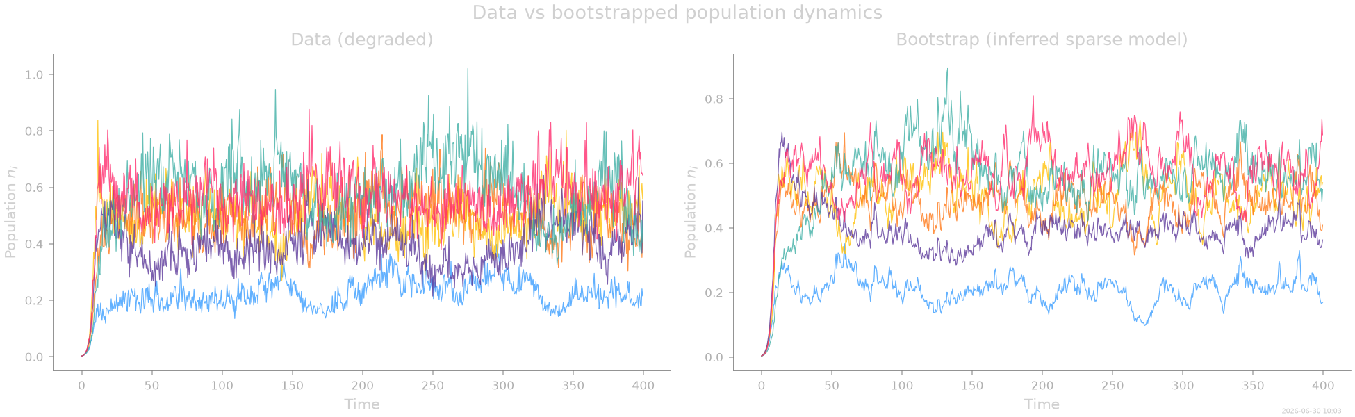
Bootstrap trajectory

Simulate a new trajectory from the inferred sparse model and compare population dynamics to the original data.

key_boot = random.PRNGKey(seed + 99)
coll_boot, _ = inf.simulate_bootstrapped_trajectory(key_boot, oversampling=oversampling)

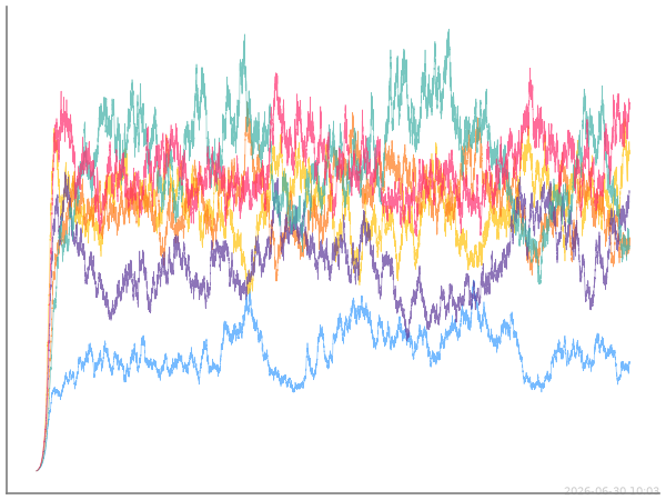
Thumbnail

Compact population time series for the gallery grid.

stamp_output()

[Generated: 2026-06-30 10:03]

🏷 Tags: synthetic, overdamped, nonlinear, sparsity, ecology, custom-basis