Note
Go to the end to download the full example code.
Anisotropic diffusion tensor field
Recover a position-dependent, anisotropic diffusion tensor \(D(\mathbf{x})\) from a single 2D trajectory — model-free. A tracer in a ring trap experiences fluctuations whose radial component grows with distance from the center (think of a probe in a radially stretched gel, or near a topological defect in an active film): the local noise ellipse rotates with position. A polynomial tensor basis recovers the full field, including its principal axes.
Tags
synthetic · overdamped · multiplicative-noise · diffusion-field · anisotropic · 2D
Model and simulation
A particle in a ring potential \(U = \tfrac{k}{4}(r^2 - R^2)^2\) with a radially anisotropic diffusion tensor (Itô convention):
Radial kicks grow with \(r\); tangential noise stays at \(D_0\). Both fields are polynomial, so we can build them compositionally from coordinate and matrix-template primitives.
import SFI
from SFI.bases import identity_matrix_basis, symmetric_matrix_basis, unit_axes, x_components
from SFI.langevin import OverdampedProcess

k = 4.0       # ring trap stiffness
R = 1.5       # ring radius
D0 = 0.2      # isotropic (tangential) diffusion
a = 0.15      # radial anisotropy growth
dt = 0.005
Nsteps = 50_000

x, y = x_components(2)
ex, ey = unit_axes(2)
I = identity_matrix_basis(2)
S = symmetric_matrix_basis(2)            # templates Sxx, Sxy, Syy
Sxx, Sxy, Syy = S[0], S[1], S[2]

r2 = x**2 + y**2
F_model = (-k * (r2 - R**2)) * (x * ex + y * ey)
D_model = D0 * I + a * (x**2 * Sxx + x * y * Sxy + y**2 * Syy)

proc = OverdampedProcess(F=F_model, D=D_model,
                         theta_F=jnp.ones(F_model.n_features),
                         theta_D=jnp.ones(D_model.n_features))
proc.initialize(jnp.array([R, 0.0]))
coll = proc.simulate(dt=dt, Nsteps=Nsteps, key=random.PRNGKey(11),
                     prerun=500, oversampling=10)
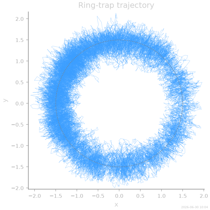
Trajectory
The tracer diffuses around the annulus, sampling all orientations of the local anisotropy.
Inference
Same canonical sequence as in 1D — the only change is the rank-2 tensor basis for the diffusion field: degree-2 matrix monomials, spanning all symmetric-tensor fields with polynomial entries (18 features; the truth uses 5 of them).
from SFI.bases import monomials_up_to

B_force = monomials_up_to(order=3, dim=2, rank="vector")
B_diff = monomials_up_to(order=2, dim=2, rank="symmetric_matrix")

inf = SFI.OverdampedLangevinInference(coll)
inf.compute_diffusion_constant()
inf.infer_force_linear(B_force)
inf.compute_force_error()
inf.infer_diffusion_linear(B_diff)

inf.compare_to_exact(model_exact=proc)
inf.print_report()
  --- StochasticForceInference Report ---
Average diffusion tensor:
 [[ 0.33276835 -0.01264946]
 [-0.01264946  0.33020318]]
Measurement noise tensor:
 [[ 1.17328607e-04 -1.01671212e-05]
 [-1.01671212e-05  1.06286105e-04]]
Force estimated information: 1458.69287109375
Force: estimated normalized mean squared error (sampling only): 0.006855446174737724
Normalized MSE (force):     0.0092
Normalized MSE (diffusion): 0.0235

  Force Coefficient Table
  ─────────────────────────────────────────────────────────────────────
  #    Label          Coefficient       Std.Err     SNR  Sig
  ─────────────────────────────────────────────────────────────────────
  0    1·e0          -9.40828e-03   2.64348e-01     0.0  ·
  1    1·e1           1.33710e-01   2.63323e-01     0.5  ·
  2    x0·e0          8.36846e+00   2.58974e-01    32.3  **
  3    x0·e1          2.15885e-01   2.57973e-01     0.8  ·
  4    x1·e0         -1.86756e-01   2.41069e-01     0.8  ·
  5    x1·e1          8.27424e+00   2.40137e-01    34.5  **
  6    x0^2·e0        2.46907e-02   1.21943e-01     0.2  ·
  7    x0^2·e1       -1.71195e-02   1.21471e-01     0.1  ·
  8    (x0·x1)·e0     1.59657e-02   7.07004e-02     0.2  ·
  9    (x0·x1)·e1     2.04636e-02   7.04274e-02     0.3  ·
  10   x1^2·e0       -3.27893e-02   1.21499e-01     0.3  ·
  11   x1^2·e1       -1.04222e-01   1.21027e-01     0.9  ·
  12   x0^3·e0       -3.70496e+00   1.10419e-01    33.6  **
  13   x0^3·e1       -1.09802e-01   1.09993e-01     1.0  ·
  14   (x0^2·x1)·e0   7.52521e-02   1.20086e-01     0.6  ·
  15   (x0^2·x1)·e1  -3.62706e+00   1.19622e-01    30.3  **
  16   (x0·x1^2)·e0  -3.71582e+00   1.26633e-01    29.3  **
  17   (x0·x1^2)·e1  -3.57414e-02   1.26144e-01     0.3  ·
  18   x1^3·e0        1.06565e-01   1.03542e-01     1.0  ·
  19   x1^3·e1       -3.69748e+00   1.03142e-01    35.8  **
  ─────────────────────────────────────────────────────────────────────
  20/20 basis functions in support, sig: 6* / 6** / 0*** (|SNR| ≥ 2 / 10 / 100)
  (Std.err. reflects sampling error only; discretization bias is not included.)
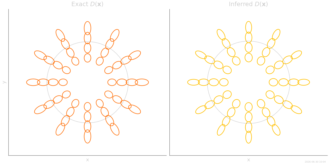
Tensor glyphs: exact vs inferred
Each glyph is the ellipse \(\mathbf{u}^{\!\top} D^{-1}\mathbf{u} = \text{const}\) of the local tensor — long axis along the fast direction. Exact field on the left, inferred on the right: the radial orientation and the \(r^2\) growth are both recovered.
# Glyph positions on a polar grid covering the sampled annulus, and a
# callable for the exact tensor field D(x) = D0 I + a r^2 r-hat r-hat^T.
r_glyph = np.linspace(0.9, 2.0, 4)
th_glyph = np.linspace(0, 2 * np.pi, 12, endpoint=False)
pts = np.array([[r * np.cos(t), r * np.sin(t)] for r in r_glyph for t in th_glyph])


def D_exact_field(p):
    p = np.asarray(p).reshape(-1, 2)
    return np.array([D0 * np.eye(2) + a * np.outer(q, q) for q in p])


def D_inferred_field(p):
    return inf.diffusion_inferred(jnp.asarray(p))
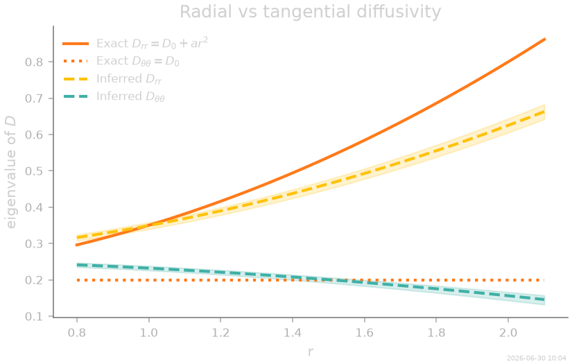
Radial and tangential eigenvalues
Projecting the inferred tensor onto the local radial and tangential directions separates the two physical components: the radial diffusivity grows as \(D_0 + a r^2\) while the tangential one stays flat at \(D_0\).
r_prof = np.linspace(0.8, 2.1, 30)
th_s = np.linspace(0, 2 * np.pi, 24, endpoint=False)
D_rr = np.zeros((len(r_prof), len(th_s)))
D_tt = np.zeros_like(D_rr)
for j, t_ in enumerate(th_s):
    pts_ray = np.column_stack([r_prof * np.cos(t_), r_prof * np.sin(t_)])
    D_ray = np.asarray(inf.diffusion_inferred(jnp.array(pts_ray)))
    rhat = np.array([np.cos(t_), np.sin(t_)])
    that = np.array([-np.sin(t_), np.cos(t_)])
    D_rr[:, j] = np.einsum("i,nij,j->n", rhat, D_ray, rhat)
    D_tt[:, j] = np.einsum("i,nij,j->n", that, D_ray, that)

#
# Shaded bands show the spread over sampling angles — a measure of how
# isotropically the basis error is distributed.  The same workflow
# applies unchanged to experimental 2D tracking data; see the
# :doc:`multiplicative-noise demo <multiplicative_diffusion_demo>` for
# the Itô-convention caveats that come with state-dependent noise.
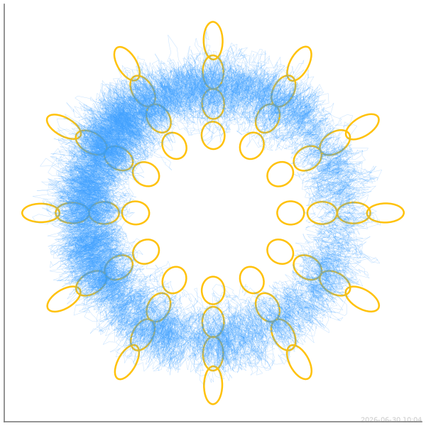
Thumbnail
Dedicated single-panel figure for the gallery thumbnail.
stamp_output()
[Generated: 2026-06-30 10:04]
Total running time of the script: (0 minutes 19.985 seconds)