Note

Go to the end to download the full example code.

Measuring dissipation: entropy production in a driven optical trap¶

synthetic overdamped linear 2D non-equilibrium thermodynamics

A colloidal bead in an optical trap looks like the textbook equilibrium system — yet real tweezers exert a small non-conservative force: the scattering force has a curl component that silently stirs the bead (Roichman et al., PRL 2008; Wu et al., PRL 2009). This demo treats that situation from the point of view of stochastic thermodynamics: the bead obeys the overdamped Langevin equation

\[\frac{\mathrm{d}\mathbf{x}}{\mathrm{d}t} = \underbrace{-k\,\mathbf{x}}_{\text{trap}} + \underbrace{\varepsilon\,(\hat z \times \mathbf{x})}_{\text{curl drive}} + \sqrt{2D}\,\boldsymbol{\xi}(t),\]

with a faint rotational drive $\varepsilon \ll k$ breaking detailed balance. The twist: the steady-state density of this driven trap is exactly the Boltzmann distribution of the trap alone — no static observable reveals the drive. Its only signatures are dynamical: a circulating probability current, and a positive entropy production rate, exactly $\sigma = 2\varepsilon^2/k$ (in units of $k_B$ per unit time) for this system.

Across this page we will:

simulate the driven trap and check that its density is Boltzmann;
infer force and diffusion, and let PASTIS find the faint curl term;
decompose the dynamics into an equilibrium part (a potential) and a drive (a current);
measure the entropy production with compute_entropy_production() and compare it to the exact rate;
ask how faint a drive is detectable — the thermodynamic limit of detection;
re-fit the model parametrized by its energy, using automatic differentiation.

The estimator is the one introduced with SFI itself (Frishman & Ronceray, PRX 2020): project the phase-space velocity onto a basis, contract with the inverse diffusion — dissipation becomes a measurable quantity of the trajectory alone.

A trap that hides its drive¶

We simulate a bead in a two-dimensional isotropic harmonic trap of stiffness $k$, plus a weak rotational force $\varepsilon\,(\hat z\times\mathbf{x})$ — the minimal model of a tweezer’s non-conservative scattering component. Units are natural ($k_BT = 1$, mobility 1): for a micron-sized bead in water, one time unit is the trap relaxation time ($\sim$ tens of ms) and lengths are in units of the thermal trap width.

The drive is faint: $\varepsilon/k = 0.3$, and we also run an equilibrium control ($\varepsilon = 0$) for comparison. One long recording — a few thousand relaxation times — will turn out to be exactly what measuring this faint dissipation requires.

import SFI
from SFI.bases import unit_axes, x_components
from SFI.langevin import OverdampedProcess

k_true = 1.0       # trap stiffness
eps_true = 0.3     # rotational drive:  F_curl = eps * (z_hat x x)
D_true = 0.5       # diffusion constant
dt = 0.01          # time between recorded frames
Nsteps = 320_000   # frames per run (3200 trap relaxation times)

x0c, x1c = x_components(2)
e0, e1 = unit_axes(2)


def make_trap(eps):
    """Isotropic trap + curl drive of amplitude eps, as a basis expression."""
    return (-k_true * x0c - eps * x1c) * e0 + (-k_true * x1c + eps * x0c) * e1


def simulate_trap(eps, seed):
    proc = OverdampedProcess(make_trap(eps), D=D_true)
    key_init, key_run = random.split(random.PRNGKey(seed))
    x_init = jnp.sqrt(D_true / k_true) * random.normal(key_init, (2,))
    proc.initialize(x_init)
    coll_run = proc.simulate(
        dt=dt, Nsteps=Nsteps, key=key_run,
        prerun=500, oversampling=4, compute_observables=True,
    )
    return coll_run, proc


coll, proc_true = simulate_trap(eps_true, seed=4)
coll_eq, _ = simulate_trap(0.0, seed=2)

sigma_exact = 2.0 * eps_true**2 / k_true
print(f"Simulated {coll.T} frames at dt = {dt}"
      f"  (total observation time {Nsteps * dt:.0f})")
print(f"Exact entropy production rate: sigma = 2 eps^2 / k = {sigma_exact:.3f} kB / time")

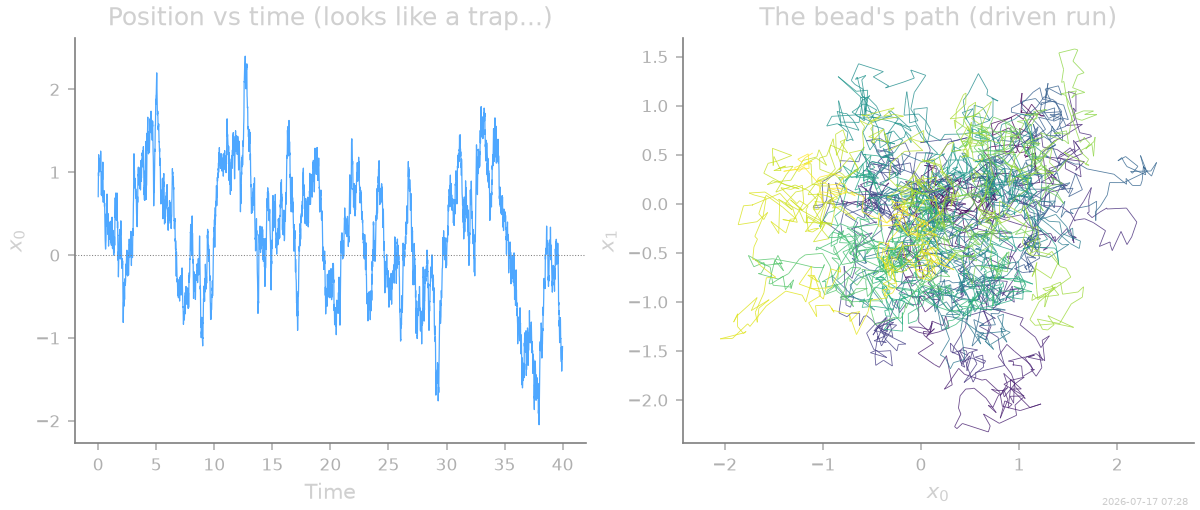
Position vs time (looks like a trap...), The bead's path (driven run)

Simulated 320000 frames at dt = 0.01  (total observation time 3200)
Exact entropy production rate: sigma = 2 eps^2 / k = 0.180 kB / time

Statics look like equilibrium¶

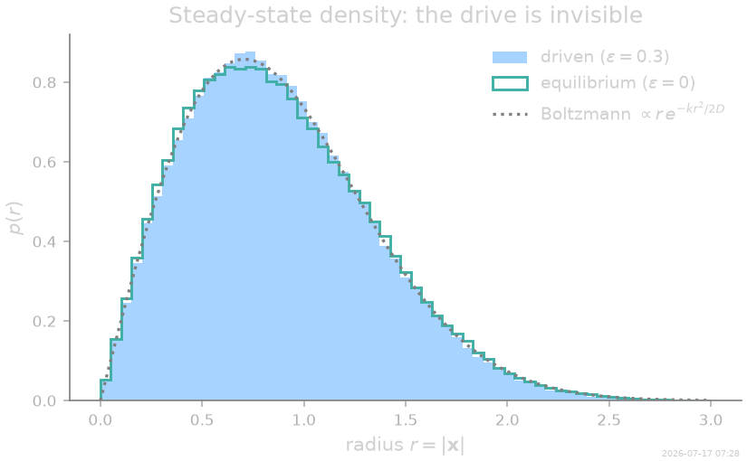
The curl force is divergence-free and everywhere tangent to the circles of constant $|\mathbf{x}|$ — so it stirs probability along the level sets of the trap’s Boltzmann density without reshaping it. The driven steady state is exactly $\rho(\mathbf{x}) \propto e^{-k|\mathbf{x}|^2/2D}$, independent of $\varepsilon$.

The radial histograms of the driven and equilibrium runs confirm it: they are statistically indistinguishable, and both match the Boltzmann prediction. Snapshots cannot reveal this non-equilibrium system — only the arrow of time in the trajectories can.

Steady-state density: the drive is invisible

Infer the dynamics¶

Standard SFI workflow: estimate the diffusion constant, then regress the force onto a deliberately over-complete polynomial basis and let PASTIS decide which terms the data support. The interesting question: does model selection keep the faint curl term?

from SFI.bases import monomials_up_to

inf = SFI.OverdampedLangevinInference(coll)
inf.compute_diffusion_constant(method="MSD")   # clean synthetic data

B = monomials_up_to(2, dim=2, rank="vector")   # 12 candidate terms
inf.infer_force_linear(B)
inf.compute_force_error()

coeffs_full = np.asarray(inf.force_coefficients_full)
stderr_full = np.asarray(inf.force_coefficients_stderr)

inf.sparsify_force(criterion="PASTIS")
inf.compute_force_error()
inf.print_report()

  --- StochasticForceInference Report ---
Average diffusion tensor:
 [[ 0.4970535  -0.00107499]
 [-0.00107499  0.49664953]]
Measurement noise tensor:
 [[ 3.3270899e-05 -1.2681787e-05]
 [-1.2681789e-05  3.7669979e-05]]
Force estimated information: 1748.693359375
Force: estimated normalized mean squared error (sampling only): 0.0011437110286194087

  Force Coefficient Table
  ───────────────────────────────────────────────────────────────────
  #    Label        Coefficient       Std.Err     SNR  Sig
  ───────────────────────────────────────────────────────────────────
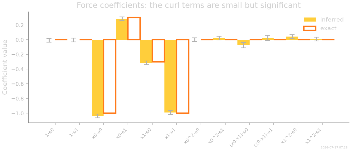
  2    x0·e0       -1.03441e+00   2.54568e-02    40.6  **
  3    x0·e1        2.85636e-01   2.54464e-02    11.2  **
  4    x1·e0       -3.16391e-01   2.50761e-02    12.6  **
  5    x1·e1       -9.90777e-01   2.50659e-02    39.5  **
  ───────────────────────────────────────────────────────────────────
  4/12 basis functions in support, sig: 4* / 4** / 0*** (|SNR| ≥ 2 / 10 / 100)
  (Std.err. reflects sampling error only; discretization bias is not included.)
  Zeroed (8): 1·e0, 1·e1, x0^2·e0, x0^2·e1, (x0·x1)·e0, (x0·x1)·e1, x1^2·e0, x1^2·e1

PASTIS retains exactly the four linear terms — the isotropic trap and the antisymmetric curl couplings, which are an order of magnitude smaller. The faint drive is not just detected: its structure is identified.

Force coefficients: the curl terms are small but significant

An equilibrium part and a drive¶

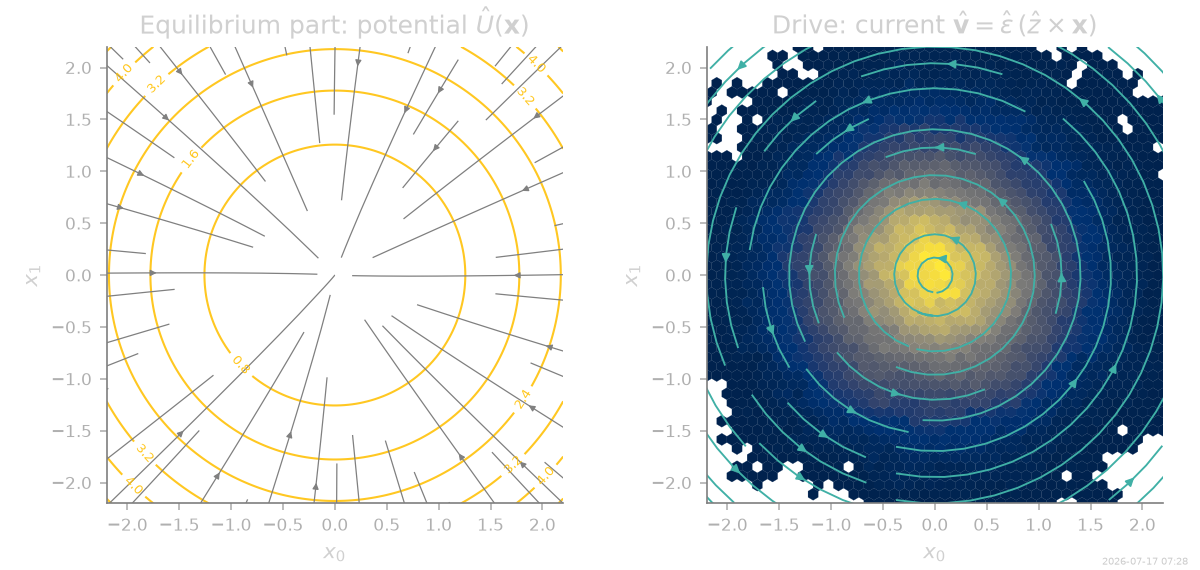
For a linear force $\mathbf{F} = M\mathbf{x}$, the symmetric part of $M$ is the (conservative) trap and the antisymmetric part is the non-conservative drive. We read $\hat M$ off the inferred force field by automatic differentiation and split it:

import jax

F_hat = lambda x: inf.force_inferred(x[None, :])[0]
M_hat = np.asarray(jax.jacobian(F_hat)(jnp.zeros(2)))

k_hat = -0.5 * (M_hat[0, 0] + M_hat[1, 1])       # trap stiffness
eps_hat = 0.5 * (M_hat[1, 0] - M_hat[0, 1])      # curl amplitude

print(f"trap stiffness : k_hat   = {k_hat:.4f}   (true {k_true})")
print(f"curl amplitude : eps_hat = {eps_hat:.4f}   (true {eps_true})")

trap stiffness : k_hat   = 1.0126   (true 1.0)
curl amplitude : eps_hat = 0.3010   (true 0.3)

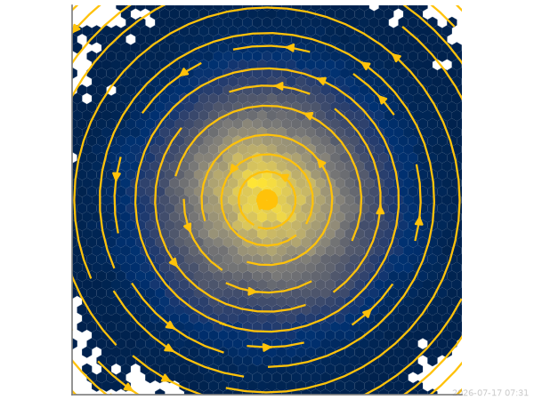
The two parts play very different thermodynamic roles. The symmetric part integrates to a potential $\hat U = \tfrac12 \hat k |\mathbf{x}|^2$ whose Boltzmann weight is the observed density. The antisymmetric part is precisely the mean local velocity $\hat{\mathbf{v}}(\mathbf{x}) = \hat\varepsilon\,(\hat z \times \mathbf{x})$ — the circulating probability current that a movie of the bead would reveal but a snapshot cannot.

Equilibrium part: potential $\hat U(\mathbf{x})$, Drive: current $\hat{\mathbf{v}} = \hat\varepsilon\,(\hat z\times\mathbf{x})$

The price of the current: entropy production¶

Maintaining that circulation costs free energy, dissipated into the bath at the entropy production rate $\sigma = \langle \mathbf{v}\cdot D^{-1}\mathbf{v}\rangle$. compute_entropy_production() estimates it directly from the fit, by projecting the phase-space velocity onto the force basis (Frishman & Ronceray, PRX 2020) — with an error bar, and a fluctuation bias $2N_b/\tau_N$ that tells you how much apparent dissipation mere noise would produce with this basis and this much data.

out = inf.compute_entropy_production()

S_sim = coll.datasets[0].meta["observables"]["entropy"]  # simulator ground truth
tauN = out["tauN"]

print(f"exact rate                    : {sigma_exact:.4f} kB / time")
print(f"inferred (projection)         : {out['Sdot']:.4f} +- {out['Sdot_error']:.4f}"
      f"   [fluctuation bias {out['Sdot_bias']:.4f}]")
print(f"from the fitted model 2e^2/k  : {2 * eps_hat**2 / k_hat:.4f}")
print(f"true model on this trajectory : {S_sim / tauN:.4f}")

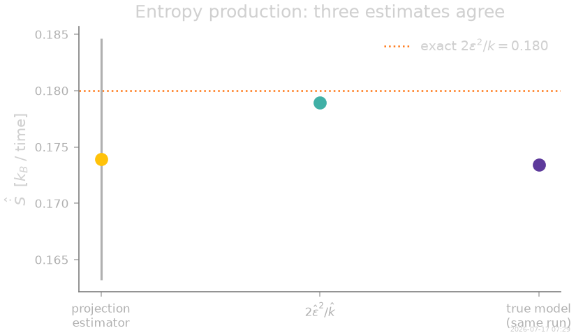
Entropy production: three estimates agree

exact rate                    : 0.1800 kB / time
inferred (projection)         : 0.1739 +- 0.0107   [fluctuation bias 0.0025]
from the fitted model 2e^2/k  : 0.1790
true model on this trajectory : 0.1734

The report now carries the dissipation too — print_report() shows Entropy production (total Delta S, estimated error) once the estimator has run. Note the estimator only uses the inferred force and diffusion: no ground truth enters. A subtlety worth naming: what is measured is the entropy produced along this trajectory, which itself fluctuates from run to run — the reported error bar includes that fluctuation (the $2\Delta\hat S$ term), which is why all three estimates track each other more tightly than they track the ensemble value.

How faint a drive can you detect?¶

Near equilibrium the current is linear in the drive, so the dissipation is quadratic: $\sigma = 2\varepsilon^2/k$. Detecting a twice-fainter drive takes four times the entropy — and the estimator’s own fluctuation bias sets the floor: irreversibility becomes detectable only once the trajectory has dissipated a few $k_B$ more than the bias $2N_b$. We sweep $\varepsilon$ at fixed trajectory length, then sweep the trajectory length at fixed faint drive.

B_lin = monomials_up_to(1, dim=2, include_constant=False, rank="vector")


def entropy_of(coll_run):
    """MSD diffusion + linear force fit + entropy production, in one go."""
    inf_run = SFI.OverdampedLangevinInference(coll_run)
    inf_run.compute_diffusion_constant(method="MSD")
    inf_run.infer_force_linear(B_lin)
    return inf_run.compute_entropy_production()


eps_sweep = [0.05, 0.1, 0.2, 0.3, 0.5, 0.8]
runs = {eps_true: coll}
for i, eps in enumerate(eps_sweep):
    if eps not in runs:
        runs[eps], _ = simulate_trap(eps, seed=10 + i)
sweep = {eps: entropy_of(runs[eps]) for eps in eps_sweep}

out_eq = entropy_of(coll_eq)
print(f"equilibrium control: Sdot = {out_eq['Sdot']:.4f} +- {out_eq['Sdot_error']:.4f}"
      f"  (bias {out_eq['Sdot_bias']:.4f})  -> consistent with zero")

equilibrium control: Sdot = 0.0003 +- 0.0025  (bias 0.0025)  -> consistent with zero

For the length sweep we truncate the $\varepsilon = 0.1$ run — dissipating only $\sigma \approx 0.02\,k_B$ per unit time — to increasingly short observation windows:

from SFI import TrajectoryCollection


def truncate(coll_run, T_keep):
    _, X_run, _ = coll_run.to_arrays(dataset=0)
    return TrajectoryCollection.from_arrays(X=jnp.asarray(X_run[:T_keep]), dt=dt)


T_sweep = [20_000, 40_000, 80_000, 160_000, 320_000]
length_sweep = [entropy_of(truncate(runs[0.1], T)) for T in T_sweep]

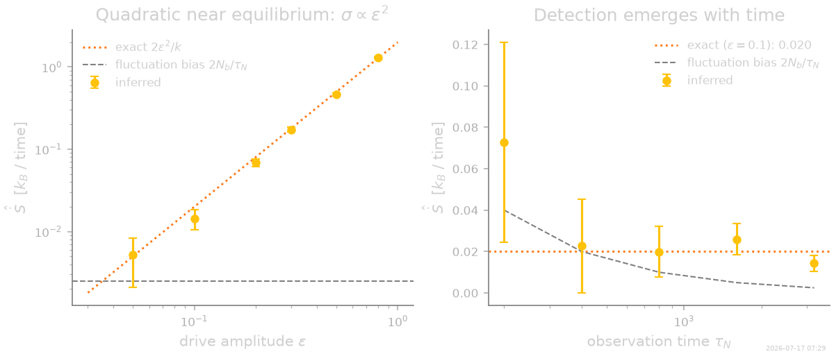
Quadratic near equilibrium: $\sigma \propto \varepsilon^2$, Detection emerges with time

The left panel shows the near-equilibrium scaling over more than two decades of dissipation, down to the detection floor where the inferred rate meets the fluctuation bias. The right panel shows detection emerging as data accumulates: with $\tau_N \lesssim 10^3$ the faint drive is buried in the bias; a few thousand relaxation times resolve it cleanly. The rule of thumb — the trajectory must dissipate a few $k_B$ beyond the $2N_b$ bias — is the thermodynamic cost of measuring irreversibility.

Fit the energy, not the force¶

Near equilibrium, the natural parametrization is thermodynamic: an energy landscape $U_\theta$ plus a drive amplitude. With SFI’s parametric estimator and JAX autodiff, we fit $\mathbf{F}_\theta = -\nabla U_\theta + \varepsilon\,(\hat z\times\mathbf{x})$ directly — here with $U_\theta = \tfrac12 k |\mathbf{x}|^2 + \tfrac14 u |\mathbf{x}|^4$, where the quartic coefficient $u$ lets the data bound the anharmonicity of the trap.

from SFI.statefunc import ParamSpec, make_psf


def U_theta(x, params):
    r2 = jnp.sum(x**2)
    return 0.5 * params["k"] * r2 + 0.25 * params["u"] * r2**2


def F_theta(x, *, params):
    return -jax.grad(U_theta)(x, params) + params["eps"] * jnp.array([-x[1], x[0]])


F_psf = make_psf(
    F_theta, dim=2, rank=1,
    params=[ParamSpec("k", shape=()), ParamSpec("u", shape=()), ParamSpec("eps", shape=())],
)

inf_energy = SFI.OverdampedLangevinInference(coll)
inf_energy.infer_force(F_psf)
inf_energy.compute_force_error()

theta = F_psf.unflatten_params(inf_energy.force_coefficients_full)
theta_err = np.asarray(inf_energy.force_coefficients_stderr)
for name, true_val, err in zip(("k", "u", "eps"), (k_true, 0.0, eps_true), theta_err):
    print(f"{name:>4s} = {float(theta[name]):+.4f} +- {err:.4f}   (true {true_val:+.3f})")

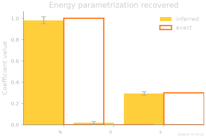
  k = +0.9824 +- 0.0321   (true +1.000)
  u = +0.0179 +- 0.0138   (true +0.000)
eps = +0.2942 +- 0.0180   (true +0.300)

The energy parameters come back with error bars: the trap stiffness and drive amplitude are recovered, and the anharmonicity is bounded — consistent with zero. Deriving forces from energies via autodiff scales to arbitrarily rich landscapes (see the Müller–Brown surface in Neural-network energy landscape — Müller-Brown potential).

Next steps¶

Theory: the estimator, its bias and error bars, the Itô-information / Stratonovich-entropy duality, and what coarse-graining does to these measurements — Stochastic thermodynamics with SFI.
Strongly driven systems: a non-equilibrium steady state with $O(1)$ currents — 2D limit cycle — nonlinear overdamped inference.
State-dependent noise breaks the naive Boltzmann picture in a different way (spurious drifts) — Multiplicative noise — the Landauer blowtorch.
Driven vs inertial: a rotational current is not inertia; the dynamics-order classifier tells them apart — Overdamped or underdamped? Classifying dynamics from data.
Real tweezer data with localization noise: Experimental-data workflow template.

Thumbnail¶

stamp_output()

[Generated: 2026-07-17 07:31]

Total running time of the script: (2 minutes 29.553 seconds)

🏷 Tags: synthetic, overdamped, linear, 2D, non-equilibrium, thermodynamics

Gallery generated by Sphinx-Gallery