Note
Go to the end to download the full example code.
Inertial dissipation: entropy production from positions only
The overdamped entropy-production demo measured the dissipation of a driven optical trap. Here the same bead keeps its inertia: the state is \((\mathbf{x}, \mathbf{v})\), the bath exerts friction and noise on the velocity,
and — crucially — only positions are observed. Underdamped Langevin Inference reconstructs the velocities, fits the full acceleration field \(F(\mathbf{x},\mathbf{v})\), and splits it by time-reversal parity (\(\mathbf{x}\) even, \(\mathbf{v}\) odd): a reversible part \(F^{+}\) (trap and drive) and an irreversible part \(F^{-}\) (friction). The entropy production is then the Stratonovich log path-probability ratio of the fitted model, evaluated on the data.
Inertia is not a detail here. For this linear system the exact rate is
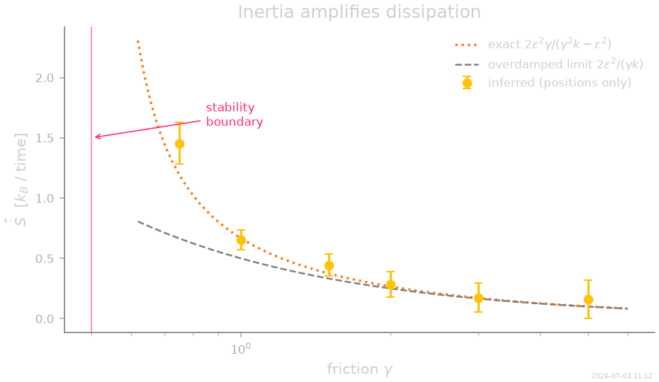
which grows as friction decreases — diverging at the stability boundary \(\gamma \to \varepsilon/\sqrt{k}\) where the curl overcomes the trap — and only settles onto the overdamped result \(2\varepsilon^2/(\gamma k)\) at strong friction. Analysing inertial data with an overdamped model misses this amplification.
Across this page we will:
simulate the inertial driven trap, recording positions only;
fit \(F(\mathbf{x},\mathbf{v})\) with ULI and let PASTIS find the trap, curl and friction terms;
split the fit by time-reversal parity with
time_reversal_split();measure the entropy production with
compute_entropy_production(), cross-check it against the simulator’s ground truth, and remove the same-sample plug-in bias by cross-fitting;sweep the friction: inertia amplifies dissipation, and the estimator tracks the exact \(\sigma(\gamma)\);
push the sampling interval past the velocity correlation time and watch the reconstruction fail — the \(\Delta t \lesssim \tau_v\) prerequisite.
Tags
synthetic · underdamped · linear · 2D · non-equilibrium · thermodynamics
An inertial bead in the driven trap
Same trap, same faint rotational drive as the overdamped page — but the bead now carries momentum (think a levitated microsphere in low-pressure gas rather than a colloid in water). We pick a moderately underdamped regime, \(\gamma = \sqrt{k}\) (quality factor near one), where the exact rate \(\sigma = 2\varepsilon^2\gamma/(\gamma^2 k - \varepsilon^2)\) is already 1.33× the overdamped formula.
The simulator integrates the phase-space dynamics but the returned
collection contains positions only — exactly what a camera sees.
compute_observables=True makes it accumulate the ground-truth
information and entropy along the way, using the true internal
velocities (which are otherwise discarded).
import SFI
from SFI.bases import unit_axes, v_components, x_components
from SFI.langevin import UnderdampedProcess

k_true = 1.0       # trap stiffness
eps_true = 0.5     # rotational drive:  F_curl = eps * (z_hat x x)
gamma_true = 1.0   # friction
D_true = 0.5       # velocity-space diffusion
dt = 0.01          # time between recorded frames
Nsteps = 320_000   # frames (3200 velocity relaxation times)

x0c, x1c = x_components(2)
v0c, v1c = v_components(2)
e0, e1 = unit_axes(2)


def make_trap(eps, gamma):
    """Trap + curl drive + friction, as a basis expression F(x, v)."""
    return (
        (-k_true * x0c - eps * x1c - gamma * v0c) * e0
        + (-k_true * x1c + eps * x0c - gamma * v1c) * e1
    )


def simulate_trap(eps, gamma, seed, *, dt=dt, Nsteps=Nsteps, oversampling=8):
    proc = UnderdampedProcess(make_trap(eps, gamma), D=D_true)
    proc.initialize(jnp.array([0.5, 0.0], dtype=jnp.float32))
    coll_run = proc.simulate(
        dt=dt, Nsteps=Nsteps, key=random.PRNGKey(seed),
        prerun=500, oversampling=oversampling, compute_observables=True,
    )
    return coll_run, proc


def sigma_exact(eps, gamma):
    return 2.0 * eps**2 * gamma / (gamma**2 * k_true - eps**2)


coll, proc_true = simulate_trap(eps_true, gamma_true, seed=3)

print(f"Simulated {coll.T} frames at dt = {dt} (positions only)")
print(f"Exact entropy production rate: sigma = {sigma_exact(eps_true, gamma_true):.4f} kB / time")
print(f"Overdamped formula would give:  {2 * eps_true**2 / (gamma_true * k_true):.4f} kB / time")
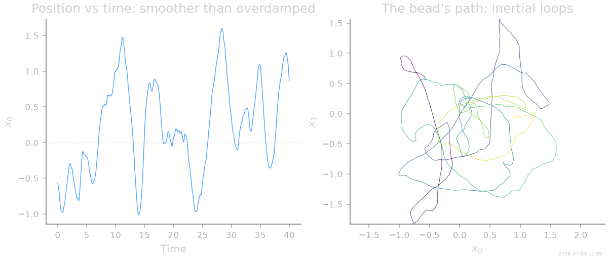
Simulated 320000 frames at dt = 0.01 (positions only)
Exact entropy production rate: sigma = 0.6667 kB / time
Overdamped formula would give:  0.5000 kB / time
Fit the acceleration field from positions
The workflow mirrors the overdamped one — the engine transparently handles the velocity reconstruction. We hand ULI an over-complete polynomial basis in \((\mathbf{x}, \mathbf{v})\) and let PASTIS decide: it should keep the linear trap terms, the faint curl, and the friction — and nothing else.
from SFI.bases import monomials_up_to

inf = SFI.UnderdampedLangevinInference(coll)
inf.compute_diffusion_constant()

B = monomials_up_to(2, dim=2, include_constant=True, include_v=True, rank="vector")
inf.infer_force_linear(B)
inf.compute_force_error()

coeffs_full = np.asarray(inf.force_coefficients_full)
stderr_full = np.asarray(inf.force_coefficients_stderr)

inf.sparsify_force(criterion="PASTIS")
inf.compute_force_error()
inf.print_report()
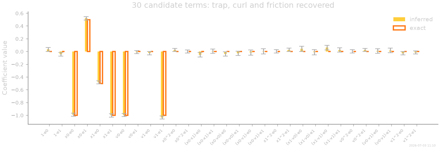
  --- StochasticForceInference Report ---
Average diffusion tensor:
 [[ 5.0369191e-01 -3.4161386e-04]
 [-3.4161386e-04  5.0351131e-01]]
Measurement noise tensor:
 [[ 5.1027321e-10 -6.0447689e-12]
 [-6.0447689e-12  3.9476983e-10]]
Force estimated information: 3711.53662109375
Force: estimated normalized mean squared error (sampling only): 0.000808290684722677

  Force Coefficient Table
  ───────────────────────────────────────────────────────────────────
  #    Label        Coefficient       Std.Err     SNR  Sig
  ───────────────────────────────────────────────────────────────────
  2    x0·e0       -1.00016e+00   2.16500e-02    46.2  **
  3    x0·e1        5.18507e-01   2.49182e-02    20.8  **
  4    x1·e0       -4.84258e-01   2.51104e-02    19.3  **
  5    x1·e1       -9.95782e-01   2.18199e-02    45.6  **
  6    v0·e0       -9.95473e-01   2.50260e-02    39.8  **
  9    v1·e1       -1.03102e+00   2.52615e-02    40.8  **
  ───────────────────────────────────────────────────────────────────
  6/30 basis functions in support, sig: 6* / 6** / 0*** (|SNR| ≥ 2 / 10 / 100)
  (Std.err. reflects sampling error only; discretization bias is not included.)
  Zeroed (24): 1·e0, 1·e1, v0·e1, v1·e0, x0^2·e0, x0^2·e1, (x0·x1)·e0, (x0·x1)·e1, (x0·v0)·e0, (x0·v0)·e1, (x0·v1)·e0, (x0·v1)·e1, x1^2·e0, x1^2·e1, (x1·v0)·e0, (x1·v0)·e1, (x1·v1)·e0, (x1·v1)·e1, v0^2·e0, v0^2·e1, (v0·v1)·e0, (v0·v1)·e1, v1^2·e0, v1^2·e1
Split the dynamics by the arrow of time
Under time reversal positions are even and velocities odd, so the fitted field splits into \(\hat F^{\pm}(\mathbf{x},\mathbf{v}) = \tfrac12[\hat F(\mathbf{x},\mathbf{v}) \pm \hat F(\mathbf{x},-\mathbf{v})]\). For this system \(\hat F^{+}\) is the trap plus the curl drive (all positional) and \(\hat F^{-}\) is the friction — the part that knows which way time flows.
F_even, F_odd = inf.time_reversal_split()

x_probe = jnp.array([[1.0, 0.0]])
v_probe = jnp.array([[0.0, 1.0]])
print("F      (x=(1,0), v=(0,1)) =", np.asarray(inf.force_inferred(x_probe, v=v_probe))[0])
print("F_even (reversible part)  =", np.asarray(F_even(x_probe, v_probe))[0])
print("F_odd  (irreversible part)=", np.asarray(F_odd(x_probe, v_probe))[0])
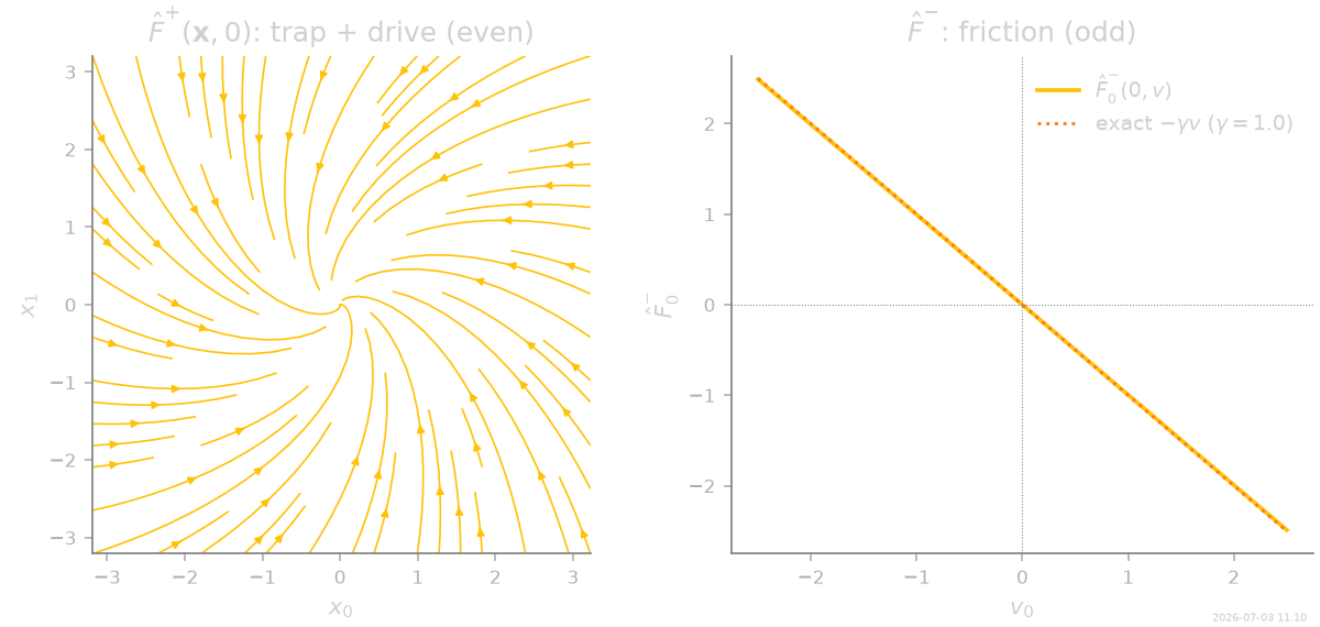
F      (x=(1,0), v=(0,1)) = [-1.0001588 -0.5125175]
F_even (reversible part)  = [-1.0001588   0.51850665]
F_odd  (irreversible part)= [ 0.        -1.0310241]
Measure the dissipation — from positions only
compute_entropy_production()
evaluates \(\Delta\hat S = \sum_t (\mathrm{d}\hat v_t \circ - \hat
F^{+}\mathrm{d}t)^\top \bar D^{-1} \hat F^{-}\) with the reconstructed
kinematics. Two subtleties, both reported by the method:
friction makes the odd sector informative but barely irreversible: the log ratio’s contributions largely cancel, so the error bar is set by the odd-sector fluctuation scale (
Q_odd), estimated analytically and by block variance;evaluating the functional with coefficients fitted on the same trajectory adds a small positive \(O(1/\tau_N)\) plug-in bias. Cross-fitting — fit on one half, evaluate on the other — removes it, via the
coefficientsargument.
out = inf.compute_entropy_production()

S_sim = coll.datasets[0].meta["observables"]["entropy"]
tauN = out["tauN"]
sigma = sigma_exact(eps_true, gamma_true)

# Cross-fitting: two halves, two fits, evaluate each on the other half.
from SFI import TrajectoryCollection

X_all = jnp.asarray(X_ud)
T_half = X_all.shape[0] // 2
halves = [
    TrajectoryCollection.from_arrays(X=X_all[:T_half], dt=dt),
    TrajectoryCollection.from_arrays(X=X_all[T_half:], dt=dt),
]
fits = []
for coll_h in halves:
    inf_h = SFI.UnderdampedLangevinInference(coll_h)
    inf_h.compute_diffusion_constant()
    inf_h.infer_force_linear(B)
    fits.append(inf_h)
out_xf = [
    fits[1].compute_entropy_production(coefficients=fits[0].force_coefficients_full),
    fits[0].compute_entropy_production(coefficients=fits[1].force_coefficients_full),
]
Sdot_crossfit = 0.5 * (out_xf[0]["Sdot"] + out_xf[1]["Sdot"])
err_crossfit = 0.5 * (out_xf[0]["Sdot_error"] ** 2 + out_xf[1]["Sdot_error"] ** 2) ** 0.5

print(f"exact rate                    : {sigma:.4f} kB / time")
print(f"inferred (same-sample)        : {out['Sdot']:.4f} +- {out['Sdot_error']:.4f}"
      f"   [odd dof bias {out['Sdot_bias']:.4f}]")
print(f"inferred (cross-fitted)       : {Sdot_crossfit:.4f} +- {err_crossfit:.4f}")
print(f"true model on this trajectory : {S_sim / tauN:.4f}")
print(f"irreversible fraction of the odd sector: {out['entropy_odd_ratio']:.3f}")
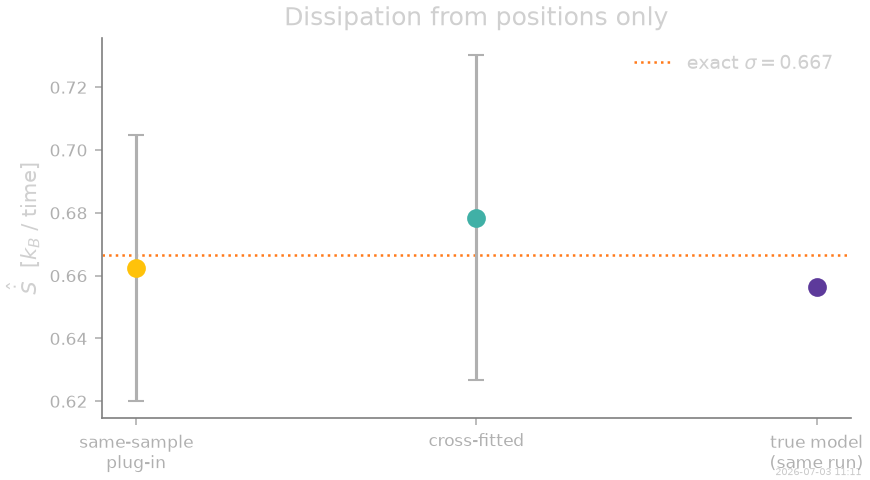
exact rate                    : 0.6667 kB / time
inferred (same-sample)        : 0.6624 +- 0.0423   [odd dof bias 0.0013]
inferred (cross-fitted)       : 0.6785 +- 0.0517
true model on this trajectory : 0.6562
irreversible fraction of the odd sector: 0.246
Inertia amplifies dissipation
Now sweep the friction at fixed drive. Watch the exact rate: far from the overdamped intuition that less friction means less dissipation, \(\sigma(\gamma)\) grows as \(\gamma\) decreases — the freely-circulating bead extracts more work from the drive — and diverges at the stability boundary \(\gamma = \varepsilon/\sqrt{k}\). The estimator, still fed positions only, tracks the exact curve; the overdamped formula (dashed) is off by 30% already at \(\gamma = 1\).
B_lin = monomials_up_to(1, dim=2, include_constant=False, include_v=True, rank="vector")


def entropy_of(coll_run):
    inf_run = SFI.UnderdampedLangevinInference(coll_run)
    inf_run.compute_diffusion_constant()
    inf_run.infer_force_linear(B_lin)
    return inf_run.compute_entropy_production()


gamma_sweep = [0.75, 1.0, 1.5, 2.0, 3.0, 5.0]
sweep = {}
for i, gam in enumerate(gamma_sweep):
    coll_g, _ = simulate_trap(eps_true, gam, seed=20 + i, Nsteps=80_000)
    sweep[gam] = entropy_of(coll_g)
When sampling is too coarse
Everything above relied on resolving the velocity correlation time \(\tau_v = 1/\gamma\). Subsampling the same recording stretches the effective \(\Delta t\); beyond \(\gamma\Delta t \approx 0.5\) the secant velocities stop resembling velocities, the estimator (which warns at exactly that threshold) degrades, and the measurement slides toward a coarse-grained lower bound. There is no free lunch: inertial dissipation is only measurable when inertia is resolved.
strides = [1, 5, 10, 20, 40, 80]
resolution = []
for s in strides:
    coll_s = TrajectoryCollection.from_arrays(X=X_all[::s], dt=dt * s)
    resolution.append((gamma_true * dt * s, entropy_of(coll_s)))

for gdt, o in resolution:
    print(f"gamma*dt = {gdt:5.2f}:  Sdot = {o['Sdot']:7.4f} +- {o['Sdot_error']:.4f}")
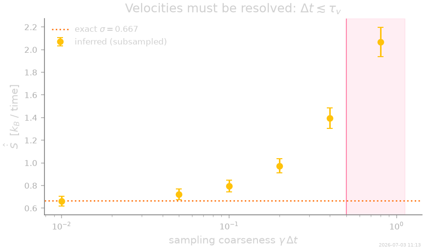
gamma*dt =  0.01:  Sdot =  0.6632 +- 0.0425
gamma*dt =  0.05:  Sdot =  0.7219 +- 0.0466
gamma*dt =  0.10:  Sdot =  0.7975 +- 0.0517
gamma*dt =  0.20:  Sdot =  0.9738 +- 0.0630
gamma*dt =  0.40:  Sdot =  1.3950 +- 0.0893
gamma*dt =  0.80:  Sdot =  2.0682 +- 0.1287
Next steps
The overdamped companion page: the same trap without inertia, the near-equilibrium detection limit, and the parametric energy fit — Measuring dissipation: entropy production in a driven optical trap.
Theory: the odd-parity split, the estimator’s provisional error bars and the cross-fitting recipe — Stochastic thermodynamics with SFI.
Driven or inertial? The dynamics-order classifier tells a rotational current from momentum — Overdamped or underdamped? Classifying dynamics from data.
Underdamped inference in depth: presets, kinematics and diagnostics — Underdamped systems.
Thumbnail
stamp_output()
[Generated: 2026-07-03 11:13]
Total running time of the script: (3 minutes 57.575 seconds)